POMDPs and Policy Gradients MLSS 2006, Canberra Douglas Aberdeen - PowerPoint PPT Presentation
POMDPs and Policy Gradients MLSS 2006, Canberra Douglas Aberdeen Canberra Node, RSISE Building Australian National University 15th February 2006 Outline Introduction 1 What is Reinforcement Learning? Types of RL Value-Methods 2 Model
POMDPs and Policy Gradients MLSS 2006, Canberra Douglas Aberdeen Canberra Node, RSISE Building Australian National University 15th February 2006
Outline Introduction 1 What is Reinforcement Learning? Types of RL Value-Methods 2 Model Based Partial Observability 3 Policy-Gradient Methods 4 Model Based Experience Based
Reinforcement Learning (RL) in a Nutshell RL can learn any function RL inherently handles uncertainty Uncertainty in actions (the world) Uncertainty in observations (sensors) Directly maximise criteria we care about RL copes with delayed feedback Temporal credit assignment problem
Reinforcement Learning (RL) in a Nutshell RL can learn any function RL inherently handles uncertainty Uncertainty in actions (the world) Uncertainty in observations (sensors) Directly maximise criteria we care about RL copes with delayed feedback Temporal credit assignment problem
Reinforcement Learning (RL) in a Nutshell RL can learn any function RL inherently handles uncertainty Uncertainty in actions (the world) Uncertainty in observations (sensors) Directly maximise criteria we care about RL copes with delayed feedback Temporal credit assignment problem
Reinforcement Learning (RL) in a Nutshell RL can learn any function RL inherently handles uncertainty Uncertainty in actions (the world) Uncertainty in observations (sensors) Directly maximise criteria we care about RL copes with delayed feedback Temporal credit assignment problem
Examples BackGammon: TD-Gammon [12] Beat the world champion in individual games Can learn things no human ever thought of! TD-Gammon opening moves now used by best humans Australian Computer Chess Champion [4] Australian Champion Chess Player RL learns the evaluation function at leaves of min-max search Elevator Scheduling [6] Crites, Barto 1996 Optimally dispatch multiple elevators to calls Not implemented as far as I know
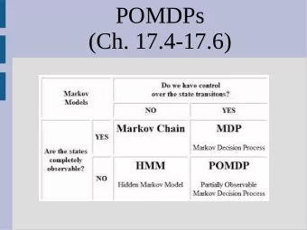
Partially Observable Markov Decision Processes world− POMDP MDP state Pr[s’|s,a] s r(s) Pr[o|s] Partial Observability RL w Pr[a|o,w] a o Agent ~ Pr[a|o,w]
Types of RL Policy POMDP MDP Value DP RL Model Based Experience
Optimality Criteria The value V ( s ) is a long-term reward from state s How do we measure long-term reward?? � ∞ � � V ∞ ( s ) = E w r ( s t ) | s 0 = s t = 0 Ill-conditioned from the decision making point of view Sum of discounted rewards � ∞ � � γ t r ( s t ) | s 0 = s V ( s ) = E w t = 0 Finite-horizon � T − 1 � � V T ( s ) = E w r ( s t ) | s 0 = s t = 0
Criteria Continued Baseline reward � ∞ � � r ( s t ) − ¯ V B ( s ) = E w r | s 0 = s t = 0 Here, ¯ r is an estimate of the Long-term average reward... Long-term average is intuitively appealing � T − 1 � � 1 ¯ V ( s ) = lim r ( s t ) | s 0 = s T E w T →∞ t = 0
Discounted or Average? Ergodic MDP Positive recurrent: finite return times Irreducible: single recurrent set of states Aperiodic: GCD of return times = 1 If the Markov system is ergodic then ¯ V ( s ) = η for all s , i.e., η is constant over s Convert from discounted to long-term average η = ( 1 − γ ) E s V ( s ) We focus on discounted V ( s ) for Value methods
Average versus Discounted V(1)=3.5 1 1 6 2 6 2 5 3 5 3 4 4 V(4)=3.5 r(s) = s V(1)=14.3 1 1 6 2 6 2 5 3 5 3 delta=0.8 4 4 V(4)=19.2
Dynamic Programming How do we compute V ( s ) for a fixed policy? Find fixed point V ∗ ( s ) solution to Bellman’s Equation: � � V ∗ ( s ) = r ( s ) + γ Pr [ s ′ | s , a ] Pr [ a | s , w ] V ∗ ( s ′ ) a ∈A s ′ ∈S In matrix form with vectors V ∗ and r : Define stochastic transition matrix for current policy � Pr [ s ′ | s , a ] Pr [ a | s , w ] P = a ∈A Now V ∗ = r + γ P V ∗ Like shortest path algs, or Viterbi estimation
Analytic Solution V ∗ = r + γ P V ∗ V ∗ − γ P V ∗ = r ( I − γ P ) V ∗ = r V ∗ = ( I − γ P ) − 1 r A x = b Computes V ( s ) for fixed policy (fixed w ) No solution unless γ ∈ [ 0 , 1 ) O ( |S| 3 ) solution... not feasible
Progress... Policy POMDP MDP TD Value SARSA Q−Learning ✁ � Value & Pol Iteration ✂ ✄ ✂ ✄ Model Based Experience
Partial Observability We have assumed so far that o = s , i.e., full observability What if s is obscured? Markov assumption violated! Ostrich approach (SARSA works well in practice) Exact methods Direct policy search: bypass values, local convergence Best policy may need full history Pr [ a t | o t , a t − 1 , o t − 1 , . . . , a 1 , o 1 ]
Belief States Belief states sufficiently summarise history b ( s ) = Pr [ s | o t , a t − 1 , o t − 1 , . . . , a 1 , o 1 ] Probability of each world state computed from history Given belief b t for time t , can update for next action � b t + 1 ( s ′ ) = ¯ b t ( s ) Pr [ s ′ | s , a t ] s ′ ∈S Now incorporate observation o t + 1 as evidence for state s ¯ b t + 1 ( s ) Pr [ o t + 1 | s ] b t + 1 ( s ) = � o ′ ∈O ¯ b t + 1 Pr [ o ′ | s ] Like HMM forward estimation Just updating the belief state is O ( |S| 2 )
Value Iteration For Belief States Do normal VI, but replace states with belief state b � � Pr [ b ′ | b , a ] Pr [ a | b , w ] V ( b ′ ) V ( b ) = r ( b ) + γ a b Expanding out terms involving b � V ( b ) = b ( s ) r ( s )+ s ∈S � � � � Pr [ s ′ | s , a ] Pr [ o | s ′ ] Pr [ a | b , w ] b ( s ) V ( b ( ao ) ) γ a ∈A o ∈O s ∈S s ′ ∈S What is V ( b ) ? l ∈L l ⊤ b V ( b ) = max
Piecewise Linear Representation common action u l 0 l 1 V(b) l 2 useless l hyperplane 3 l 4 b =1 − b 1 0 Belief state space
Policy-Graph Representation common action u l 0 l 1 V(b) l 2 l 3 l 4 b =1 − b 1 0 observation 2 a=1 a=2 a=3 observation 1 a=1
Complexity High Level Value Iteration for POMDPs Initialise b 0 (uniform/set state) 1 Receive observation o 2 Update belief state b 3 Find maximising hyperplane l for b 4 Choose action a 5 Generate new l for each observation and future action 6 While not converged, goto 2 7 Specifics generate lots of algorithms Number of hyperplanes grows exponentially: P-space hard Infinite horizon problems might need infinite hyperplanes
Approximate Value Methods for POMDPs Approximations usually learn value of representative belief states and interpolate to new belief states Belief space simplex corners are representative states Most Likely State heuristic (MLS) Q ( b , a ) = arg max Q ( b ( s ) , a ) s Q MDP assumes true state is known after one more step � Q ( b , a ) = b ( s ) Q ( s , a ) s ∈S Grid Methods distribute many belief states uniformly [5]
Progress... Policy SARSA? Exact VI ✂ ✝ ✞ ✄ POMDP MDP TD Value SARSA Q−Learning ✁ � Value & Pol Iteration ☎ ✆ ☎ Model Based Experience
Policy-Gradient Methods We all know what gradient ascent is? Value-gradient method: TD with function approximation Policy-gradient methods learn the policy directly by estimating the gradient of a long-term reward measure with respect to the parameters w that describe the policy Are there non-gradient direct policy methods? Search in policy space [10] Evolutionary algorithms [8] For the slides we give up the idea of belief states and work with observations o , i.e., Pr [ a | o , w ]
Why Policy-Gradient Pro’s No divergence, even under function approximation Occams Razor: policies are much simpler to represent Consider using a neural network to estimate a value, compared to choosing an action Partial observability does not hurt convergence (but of course, the best long-term value might drop) Are we trying to learn Q ( 0 , left ) = 0 . 255, Q ( 0 , right ) = 0 . 25 Or Q ( 0 , left ) > Q ( 0 , right ) Complexity independent of |S|
Why Not Policy-Gradient Con’s Lost convergence to the globally optimal policy Lost the Bellman constraint → larger variance Sometimes the values carry meaning
Long-Term Average Reward Recall the long-term average reward � T − 1 � � 1 ¯ V ( s ) = lim r ( s t ) | s 0 = s T E w T →∞ t = 0 And if the Markov system is ergodic then ¯ V ( s ) = η for all s We will now assume a function approximation setting We want to maximise η ( w ) by computing its gradient � ∂η � , . . . , ∂η ∇ η ( w ) = w 1 w P and stepping the parameters in that direction. For example (but there are better ways to do it): w t + 1 = w t + α ∇ η ( w )
Computing the Gradient Recall the reward column vector r An ergodic system has a unique stationary distribution of states π ( w ) So η ( w ) = π ( w ) ⊤ r Recall the state transition matrix under the current policy is � Pr [ s ′ | s , a ] Pr [ a | s , w ] P ( w ) = a ∈A So π ( w ) ⊤ = π ( w ) ⊤ P ( w )
Computing the Gradient Cont. We drop the explicit dependencies on w Let e be a column vector of 1’s The Gradient of the Long-Term Average Reward ∇ η = π ⊤ ( ∇ P )( I − P + e π ⊤ ) − 1 r Exercise: derive this expression using η = π ⊤ r and π ⊤ = π ⊤ P 1 Start with ∇ η = ( ∇ π ⊤ ) r , and ∇ π ⊤ = ( ∇ π ⊤ ) P + π ⊤ ( ∇ P ) 2 ( I − P ) is not invertible, but ( I − P + e π ⊤ ) is 3 ( ∇ π ⊤ ) e = 0 4
Recommend
More recommend
Explore More Topics
Stay informed with curated content and fresh updates.
