Outline Last time Image gradients Seam carving gradients as - PDF document
CS 376 Spring 2018 - Lecture 4 1/30/2018 Outline Last time Image gradients Seam carving gradients as energy Edges and binary images Today Tues Jan 30, 2018 Gradients edges and contours Kristen Grauman
CS 376 Spring 2018 - Lecture 4 1/30/2018 Outline • Last time – Image gradients – Seam carving – gradients as “energy” Edges and binary images • Today Tues Jan 30, 2018 – Gradients edges and contours Kristen Grauman – Template matching UT-Austin • Image patch as a filter – Binary image analysis • Blobs and regions Gradients -> edges Thresholding • Choose a threshold value t Primary edge detection steps: • Set any pixels less than t to zero (off) 1. Smoothing: suppress noise • Set any pixels greater than or equal to t to one (on) 2. Edge enhancement: filter for contrast 3. Edge localization Determine which local maxima from filter output are actually edges vs. noise • Threshold, Thin Original image Gradient magnitude image 1
CS 376 Spring 2018 - Lecture 4 1/30/2018 Thresholding gradient with a lower threshold Thresholding gradient with a higher threshold Canny edge detector The Canny edge detector • Filter image with derivative of Gaussian • Find magnitude and orientation of gradient • Non-maximum suppression : – Thin wide “ridges” down to single pixel width • Linking and thresholding ( hysteresis ): – Define two thresholds: low and high – Use the high threshold to start edge curves and the low threshold to continue them • MATLAB: edge(image, ‘canny’); original image (Lena) • >>help edge Source: D. Lowe, L. Fei-Fei Slide credit: Steve Seitz The Canny edge detector The Canny edge detector norm of the gradient thresholding 2
CS 376 Spring 2018 - Lecture 4 1/30/2018 The Canny edge detector Non-maximum suppression How to turn these thick regions of the gradient into curves? Check if pixel is local maximum along gradient direction, select single max across width of the edge thresholding • requires checking interpolated pixels p and r The Canny edge detector Problem: pixels along this edge didn’t survive the thresholding thinning (non-maximum suppression) Credit: James Hays Hysteresis thresholding • Use a high threshold to start edge curves, and a low threshold to continue them. Source: Steve Seitz Credit: James Hays 3
CS 376 Spring 2018 - Lecture 4 1/30/2018 Recap: Canny edge detector Low-level edges vs. perceived contours • Filter image with derivative of Gaussian • Find magnitude and orientation of gradient • Non-maximum suppression : – Thin wide “ridges” down to single pixel width • Linking and thresholding ( hysteresis ): – Define two thresholds: low and high – Use the high threshold to start edge curves and the low threshold to continue them • MATLAB: edge(image, ‘canny’); Shadows • >>help edge Background Texture Source: D. Lowe, L. Fei-Fei Low-level edges vs. perceived contours human segmentation image gradient magnitude Berkeley segmentation database: http://www.eecs.berkeley.edu/Research/Projects/CS/vision/grouping/segbench/ Berkeley Segmentation Data Set Credit: David Martin Source: L. Lazebnik David Martin, Charless Fowlkes, Doron Tal, Jitendra Malik 4
CS 376 Spring 2018 - Lecture 4 1/30/2018 Learn from humans which combination of features is most indicative of a “good” contour? Human-marked segment boundaries [D. Martin et al. PAMI 2004] What features are responsible for What features are responsible for perceived edges? perceived edges? Feature profiles Feature profiles (oriented energy, (oriented energy, brightness, color, brightness, color, and texture and texture gradients) along gradients) along the patch’s the patch’s horizontal horizontal diameter diameter [D. Martin et al. PAMI 2004] [D. Martin et al. PAMI 2004] Kristen Grauman, UT-Austin Kristen Grauman, UT-Austin Credit: David Martin [D. Martin et al. PAMI 2004] Kristen Grauman, UT-Austin 5
CS 376 Spring 2018 - Lecture 4 1/30/2018 Contour Detection Recall: image filtering Canny+opt thresholds Human • Compute a function of the local neighborhood at agreement Canny each pixel in the image – Function specified by a “filter” or mask saying how to Prewitt, Learned Sobel, combine values from neighbors. with Roberts combined features • Uses of filtering: – Enhance an image (denoise, resize, etc) – Extract information (texture, edges, etc) – Detect patterns (template matching) UC Berkeley Source: Jitendra Malik: Computer Vision Group http://www.cs.berkeley.edu/~malik/malik-talks-ptrs.html Adapted from Derek Hoiem Filters for features Template matching • Map raw pixels to an • Filters as templates : intermediate representation that Note that filters look like the effects they are intended to find --- “matched filters” will be used for subsequent processing • Goal: reduce amount of data, discard redundancy, preserve • Use normalized cross-correlation score to find a what’s useful given pattern (template) in the image. • Normalization needed to control for relative brightnesses. Template matching Template matching Template Template (mask) Scene Detected template A toy example 6
CS 376 Spring 2018 - Lecture 4 1/30/2018 Template matching Where’s Waldo? Template Detected template Correlation map Scene Where’s Waldo? Where’s Waldo? Template Detected template Correlation map Detected template Template matching Template matching Template Template Scene Detected template What if the template is not identical to some Match can be meaningful, if scale, orientation, and general appearance is right. subimage in the scene? How to find at any scale? 7
CS 376 Spring 2018 - Lecture 4 1/30/2018 Recap: Mask properties Summary so far • Smoothing – Values positive • Image gradients – Sum to 1 constant regions same as input • Seam carving – gradients as “energy” – Amount of smoothing proportional to mask size – Remove “high-frequency” components; “low-pass” filter • Gradients edges and contours • Derivatives • Template matching – Opposite signs used to get high response in regions of high contrast – Image patch as a filter – Sum to 0 no response in constant regions – High absolute value at points of high contrast • Filters act as templates • Highest response for regions that “look the most like the filter” • Dot product as correlation Next Motivation • Edge detection and matching – process the image gradient to find curves/contours – comparing contours • Binary image analysis – blobs and regions Figure from Belongie et al. Chamfer distance Chamfer distance • Average distance to nearest feature I Set of points in image T Set of points on (shifted) template d I ( t ) Minimum distance between point t and some point in I 8
CS 376 Spring 2018 - Lecture 4 1/30/2018 Chamfer distance Distance transform • Average distance to nearest feature Distance Transform Image features (2D) 1 0 1 2 3 4 3 2 How is the measure 1 0 1 2 3 3 2 1 different than just 1 0 1 2 3 2 1 0 1 0 0 1 2 1 0 1 filtering with a mask 2 1 1 2 1 0 1 2 having the shape 3 2 2 2 1 0 1 2 points? 4 3 3 2 1 0 1 2 5 4 4 3 2 1 0 1 How expensive is a naïve implementation? Distance Transform is a function that for each image D ( ) pixel p assigns a non-negative number corresponding to D ( p ) distance from p to the nearest feature in the image I Edge image Features could be edge points, foreground points,… Source: Yuri Boykov Distance transform (1D) Distance transform // 0 if j is in P , infinity otherwise edges original distance transform Value at (x,y) tells how far that position is from the nearest edge point (or other binary mage structure) >> help bwdist Adapted from D. Huttenlocher Chamfer distance Distance Transform (2D) • Average distance to nearest feature Edge image Distance transform image Adapted from D. Huttenlocher 9
CS 376 Spring 2018 - Lecture 4 1/30/2018 Chamfer distance Chamfer distance: properties • Sensitive to scale and rotation • Tolerant of small shape changes, clutter • Need large number of template shapes • Inexpensive way to match shapes Edge image Distance transform image Fig from D. Gavrila, DAGM 1999 Chamfer matching system Chamfer matching system • Gavrila et al. • Gavrila et al. http://gavrila.net/Research/Chamfer_System/chamfer_system.html http://gavrila.net/Research/Chamfer_System/chamfer_system.html Binary images Today • Edge detection and matching – process the image gradient to find curves/contours – comparing contours • Binary image analysis – blobs and regions 10
Recommend
More recommend
Explore More Topics
Stay informed with curated content and fresh updates.
