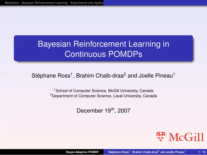
Bayesian Reinforcement Learning in Continuous POMDPs Stphane Ross 1 - PowerPoint PPT Presentation

Motivation Bayesian Reinforcement Learning Experiments and Applications Conclusion Bayesian Reinforcement Learning in Continuous POMDPs Stéphane Ross 1 , Brahim Chaib-draa 2 and Joelle Pineau 1 1 School of Computer Science, McGill University, Canada 2 Department of Computer Science, Laval University, Canada December 19 th , 2007 Stéphane Ross 1 , Brahim Chaib-draa 2 and Joelle Pineau 1 Bayes-Adaptive POMDP 1 / 18

Motivation Bayesian Reinforcement Learning Experiments and Applications Conclusion Motivation How should robots make decisions when : Environment is partially observable and continuous Poor model of sensors and actuators Parts of the model has to be learnt entirely during execution (e.g. users’ preferences/behavior) such as to maximize expected long-term rewards ? Typical Examples : [Rottmann] Solution : Bayesian Reinforcement Learning ! Stéphane Ross 1 , Brahim Chaib-draa 2 and Joelle Pineau 1 Bayes-Adaptive POMDP 2 / 18

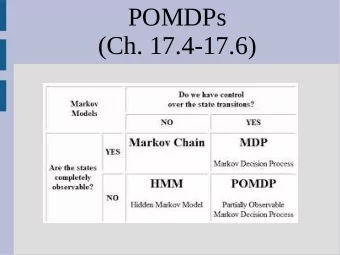
Motivation Bayesian Reinforcement Learning Experiments and Applications Conclusion Partially Observable Markov Decision Processes POMDP : ( S , A , T , R , Z , O , γ, b 0 ) S : Set of states A : Set of actions T ( s , a , s ′ ) = Pr ( s ′ | s , a ) , the transition probabilities R ( s , a ) ∈ R , the immediate rewards Z : Set of observations O ( s ′ , a , z ) = Pr ( z | s ′ , a ) , the observation probabilities γ : discount factor b 0 : Initial state distribution Belief monitoring via Bayes rule : b t ( s ′ ) = η O ( s ′ , a t − 1 , z t ) � s ∈ S T ( s , a t − 1 , s ′ ) b t − 1 ( s ) Value function : V ∗ ( b ) = max a ∈ A z ∈ Z Pr ( z | b , a ) V ∗ ( τ ( b , a , z )) � R ( b , a ) + γ � � Stéphane Ross 1 , Brahim Chaib-draa 2 and Joelle Pineau 1 Bayes-Adaptive POMDP 3 / 18

Motivation Bayesian Reinforcement Learning Experiments and Applications Conclusion Bayesian Reinforcement Learning General Idea : Define prior distributions over all unknown parameters. Maintain posteriors via Baye’s rule as experience is acquired. Plan considering posterior distribution over model. Allows us to : Learn the system at same time we achieve the task efficiently. Tradeoff optimally exploration and exploitation. Consider model uncertainty during planning. Include prior knowledge explicitly. Stéphane Ross 1 , Brahim Chaib-draa 2 and Joelle Pineau 1 Bayes-Adaptive POMDP 4 / 18

Motivation Bayesian Reinforcement Learning Experiments and Applications Conclusion Bayesian RL in Finite MDPs In Finite MDPs ( T unknown) : ([Dearden 99], [Duff 02], [Poupart 06]) → s ′ observed, a To learn T : Maintain counts φ a ss ′ of number of times s starting from prior φ 0 . Counts define Dirichlet prior/posterior over T . Planning according to φ is a MDP problem itself : S ′ : physical state ( s ∈ S ) + information state ( φ ) T ′ ( s , φ, a , s ′ , φ ′ ) Pr ( s ′ , φ ′ | s , φ, a ) = Pr ( s ′ | s , φ, a ) Pr ( φ ′ | φ, s , a , s ′ ) = φ a ss ′′ I ( φ ′ , φ + δ a = ss ′ ss ′ ) s ′′∈ S φ a � φ a � � V ∗ ( s , φ ) = max a ∈ A ss ′′ V ∗ ( s ′ , φ + δ a R ( s , a ) + γ � ss ′ ss ′ ) s ′′∈ S φ a s ′ ∈ S � Stéphane Ross 1 , Brahim Chaib-draa 2 and Joelle Pineau 1 Bayes-Adaptive POMDP 5 / 18

Motivation Bayesian Reinforcement Learning Experiments and Applications Conclusion Bayesian RL in Finite POMDPs In Finite POMDPs ( T , O unknown) : ([Ross 07]) Let : → s ′ observed. a φ a ss ′ : number of times s ψ a sz : number of times z observed in s after doing a . Given action-observation sequence, use Bayes rule to maintain belief over ( s , φ, ψ ) . ⇒ Decision under partial observability of ( s , φ, ψ ) is a POMDP itself : S ′ : physical state ( s ∈ S ) + information state ( φ, ψ ) P ′ ( s , φ, ψ, a , s ′ , φ ′ , ψ ′ , z ) = Pr ( s ′ , φ ′ , ψ ′ , z | s , φ, ψ, a ) Pr ( s ′ | s , φ, a ) Pr ( z | ψ, s ′ , a ) Pr ( φ ′ | φ, s , a , s ′ ) Pr ( ψ ′ | ψ, a , s ′ , z ) = φ a ψ a s ′ z ′ I ( φ ′ , φ + δ a ss ′ ) I ( ψ ′ , ψ + δ a = ss ′ s ′ z s ′ z ) � s ′′∈ S φ a � z ′∈ Z ψ a ss ′′ Stéphane Ross 1 , Brahim Chaib-draa 2 and Joelle Pineau 1 Bayes-Adaptive POMDP 6 / 18

Motivation Bayesian Reinforcement Learning Experiments and Applications Conclusion Example Tiger domain with unknown sensor accuracy : Suppose prior ψ 0 = ( 5 , 3 ) , b 0 = ( 0 . 5 , 0 . 5 ) Sequence of action-observation is : { (Listen,l), (Listen,l), (Listen,l), (Right,-) } 4 b 0 (L, ⋅ ) b 0 : Pr ( L , < 5 , 3 > ) = 1 2 b 3 (L, ⋅ ) Pr ( R , < 5 , 3 > ) = 1 2 3 b 3 (R, ⋅ ) b 1 : Pr ( L , < 6 , 3 > ) = 5 8 Pr ( R , < 5 , 4 > ) = 3 b 4 (L, ⋅ ) 8 2 b 3 : Pr ( L , < 8 , 3 > ) = 7 9 Pr ( R , < 5 , 6 > ) = 2 9 1 7 b 4 : Pr ( L , < 8 , 3 > ) = 18 2 Pr ( L , < 5 , 6 > ) = 18 0 7 0 0.2 0.4 0.6 0.8 1 Pr ( R , < 8 , 3 > ) = 18 accuracy 2 Pr ( R , < 5 , 6 > ) = 18 Stéphane Ross 1 , Brahim Chaib-draa 2 and Joelle Pineau 1 Bayes-Adaptive POMDP 7 / 18

Motivation Bayesian Reinforcement Learning Experiments and Applications Conclusion Continuous Domains In robotics, continuous domains are common (continuous state, continuous action, continuous observations). Could discretize the problem and apply our current method, but : Combinatorial explosion or poor precision Can require lots of training data (visit every small cell) Can we extend Bayesian RL to continuous domains ? Stéphane Ross 1 , Brahim Chaib-draa 2 and Joelle Pineau 1 Bayes-Adaptive POMDP 8 / 18

Motivation Bayesian Reinforcement Learning Experiments and Applications Conclusion Bayesian RL in Continuous Domains ? Can’t use counts (Dirichlet distribution) to learn about the model. We assume a parametric form for transtion and observation model. For instance, in the Gaussian case : S ⊂ R m , A ⊂ R n , Z ⊂ R p s t + 1 = g T ( s t , a t , X t ) z t + 1 = g O ( s t + 1 , a t , Y t ) where X t ∼ N ( µ X , Σ X ) , Y t ∼ N ( µ Y , Σ Y ) , and g T , g O are arbitrary functions (possibly non-linear). We assume g T , g O are known, but that the parameters µ X , Σ X , µ Y , Σ Y are unknown. Relevant statistics depends on the parametric form. Stéphane Ross 1 , Brahim Chaib-draa 2 and Joelle Pineau 1 Bayes-Adaptive POMDP 9 / 18

Motivation Bayesian Reinforcement Learning Experiments and Applications Conclusion Bayesian RL in Continuous Domains ? µ, Σ can be learned by maintaining sample mean ˆ µ and sample covariance ˆ Σ . These define a Normal-Wishart posterior over µ, Σ : µ, R µ | Σ = R ∼ N (ˆ ν ) Σ − 1 ∼ Wishart ( α, τ − 1 ) where : ν : number of observations for ˆ µ α : degree of freedom of ˆ Σ τ = α ˆ Σ These can be updated easily after observation X = x : α ′ = α + 1 µ ′ = ν ˆ µ + x ˆ ν + 1 τ ′ = τ + ν ′ = ν + 1 ν µ − x ) T ν + 1 (ˆ µ − x )(ˆ Stéphane Ross 1 , Brahim Chaib-draa 2 and Joelle Pineau 1 Bayes-Adaptive POMDP 10 / 18

Motivation Bayesian Reinforcement Learning Experiments and Applications Conclusion Bayesian RL in Continuous POMDP Let’s define φ = (ˆ µ X , ν X , α X , τ X ) : the posterior over ( µ X , Σ X ) ψ = (ˆ µ Y , ν Y , α Y , τ Y ) : the posterior over ( µ Y , Σ Y ) U : the update function of φ , ψ , i.e. U ( φ, x ) = φ ′ and U ( ψ, y ) = ψ ′ Bayes-Adaptive Continuous POMDP : ( S ′ , A ′ , Z ′ , P ′ , R ′ ) S ′ = S × R | X | + | X | 2 + 2 × R | Y | + | Y | 2 + 2 A ′ = A Z ′ = Z P ′ ( s , φ, ψ, a , s ′ , φ ′ , ψ ′ , z ) = I ( g T ( s , a , x ) , s ′ ) I ( g O ( s ′ , a , y ) , z ) I ( φ ′ , U ( φ, x )) I ( ψ ′ , U ( ψ, y )) f X | φ ( x ) f Y | ψ ( y ) R ′ ( s , φ, ψ, a ) = R ( s , a ) µ ′ µ ′ where x = ( ν X + 1 )ˆ X − ν X ˆ µ X and y = ( ν Y + 1 )ˆ Y − ν Y ˆ µ Y . Stéphane Ross 1 , Brahim Chaib-draa 2 and Joelle Pineau 1 Bayes-Adaptive POMDP 11 / 18

Motivation Bayesian Reinforcement Learning Experiments and Applications Conclusion Bayesian RL in Continuous POMDP Monte Carlo Belief monitoring : (1 extra assumption : g O ( s , a , · ) is 1-1 transformation of Y ) Sample ( s , φ, ψ ) ∼ b t 1 Sample ( µ X , Σ X ) ∼ NW ( φ ) 2 Sample X ∼ N ( µ X , Σ X ) 3 Compute s ′ = g T ( s , a t , X ) 4 Find unique Y s.t. 5 z t + 1 = g O ( s ′ , a t , Y ) Compute φ ′ = U ( φ, X ) , 6 ψ ′ = U ( ψ, Y ) Sample ( µ Y , Σ Y ) ∼ NW ( ψ ) 7 Add f ( Y | µ Y , Σ Y ) to particle 8 b t + 1 ( s ′ , φ ′ , ψ ′ ) Repeat until K particles in 9 b t + 1 Stéphane Ross 1 , Brahim Chaib-draa 2 and Joelle Pineau 1 Bayes-Adaptive POMDP 12 / 18

Motivation Bayesian Reinforcement Learning Experiments and Applications Conclusion Bayesian RL in Continuous POMDP Monte Carlo Online Planning (Receding Horizon Control) : b 0 a 1 a 2 a n ... o 1 o 2 o n ... b 1 b 2 b 3 Stéphane Ross 1 , Brahim Chaib-draa 2 and Joelle Pineau 1 Bayes-Adaptive POMDP 13 / 18

Motivation Bayesian Reinforcement Learning Experiments and Applications Conclusion Experiments Simple Robot Navigation Task : S : ( x , y ) position A : ( v , θ ) (velocity v ∈ [ 0 , 1 ] and angle θ ∈ [ 0 , 2 π ] ) Z : Noisy ( x , y ) position � cos θ � − sin θ g T ( s , a , X ) = s + v X sin θ cos θ g O ( s ′ , a , Y ) = s ′ + Y R ( s , a ) = I ( || s − s GOAL || 2 < 0 . 25 ) γ = 0 . 85 Stéphane Ross 1 , Brahim Chaib-draa 2 and Joelle Pineau 1 Bayes-Adaptive POMDP 14 / 18