Solving POMDPs through Macro Decomposition Larry Bush Tony Jimenez - PDF document

Solving POMDPs through Macro Decomposition Larry Bush Tony Jimenez Brian Bairstow POMDPs are a planning technique that accounts for uncertainty in the world. While they have potential, they are very computationally complex. Macro operators can reduce this complexity. 1

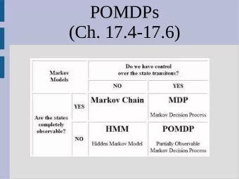
Outline • Introduction to POMDPs – Brian Bairstow • Demonstration of POMDPs – Larry Bush • Approximating POMDPs with Macro Actions – Tony Jimenez We will begin with an overview of MDP and POMDPs, and then a visual demonstration of simple MDPs and POMDPs. Finally we will discuss our advanced topic in POMDPS: the approximation of POMDPs using macro actions. 2

Introduction to POMDPs • Introduction to POMDPs – Markov Decision Processes (MDPs) – Value Iteration – Partially Observable Markov Decision Processes (POMDPs) – Overview of Techniques • Demonstration of POMDPs • Approximating POMDPs with Macro Actions Begin with completely observable Markov Decision Processes, or MDPs. Then discuss value iteration as a method of solving MDPs. This will lay the groundwork for Partially Observable Markov Decision Processes, or POMDPs. Finally there will be an overview of methods for solving POMDPs. 3

Navigation of a Building • Robot – Knows building map – Wants to reach goal – Uncertainty in actions – What is the best way to get there? Imagine a robot (in the lower right of the graphic) trying to navigate a building. It wants to reach a goal (the star in the graphic). It has difficulties in that there are uncertainties in its actions, for example its wheels could slip or catch. This might cause it to run into a wall, which is undesirable. The problem then is to find the best way to reach the goal while dealing with the problem of uncertainty in actions. How can we solve this problem? 4

Markov Decision Processes • Model • Process – States, S – Observe state s t in S – Actions, A – Choose action a t in A – Transition – Receive reward r t = r(s t ,a t ) Probabilities, p(s,a) – State becomes s t+1 according to – Rewards, r(s,a) probabilities p(s,a) • Goal – Create a policy π for choosing actions that maximizes the lifetime reward • Discount Factor γ Value = r 0 + γ r 1 + γ 2 r 2 + … We can use a MDP to solve the previous problem. An MDP consists of a model with states, actions, transitions, and expected rewards. The states in the previous problem could be positions on the map. States are discrete, so the map would have to be divided into a grid or something similar. The actions then could be to move north, east, south, or west on the map. The transition probabilities tell you the chances that a certain action from a certain state takes you to different other states. For instance, if the robot was commanded to move north, there might be a large probability that it transitions to the next state north, and small probabilities it ends up east, west, or not move at all. The reward function tells you the expected reward received by taking an action from a state. In the previous problem this could be a large reward for reaching the goal, and a large negative reward for hitting a wall. The process in carrying out an MDP solution is to observe the state in time step t, to choose an appropriate action, to receive the reward corresponding to that state and action, and to change the state according to the transition probabilities. Note that the robot is in exactly one state at a time, that time is discrete, and all actions take one time step. The goal in solving an MDP is to create a policy (a method for choosing actions) that maximizes the expected lifetime reward. The lifetime reward is the sum of all rewards received. Thus a policy should not always maximize immediate reward, but also plan ahead. Future rewards are discounted by a factor for each time step they are in the future. This follows an economic principle of the effect of time on values. Also, this makes the math work in calculating lifetime reward. Without discounting, it could be possible to receive a small reward over and over to get an infinite reward, and this is not useful in choosing a policy. A typical discount factor might be 0.9. 5

MDP Model Example p = 0.3 p = 0.4 r = 1 2 p = 0.7 r = 1 r = 0.2 r = 0 p = 0.6 1 r = 0.2 A B C p = 0.5 2 r = 1 p = 0.5 r = 0 r = 1 1 p = 0.7 p = 0.3 • States A, B, C • Actions 1, 2 • Transition probabilities p and rewards r in diagram • C is terminal state This is a simple example of an MDP model (unrelated to the previous robot example). There are 3 states and two actions. The probabilities and rewards are written in the diagram. For example, from state A, if action 1 is chosen then there is a 70% chance of staying in state A with 0 reward, and a 30% chance of moving to state C with 1 reward. State C is the terminal state, since there are no actions that move out of state C. 6

Decision Tree Representation of MDP Max Q Value Expected Reward Reward A 0.7 0 1 C 0.3 0.3 1 A 0.52 B 0.6 0.2 2 0.4 C 0.52 1 A Decision tree is another form of visualization, and allows you to evaluate the values of states. Here is a 1 step horizon decision tree for the simple model shown. From the starting point A there are two actions, 1 and 2. The action chosen gives probabilities of moving to different states. Notice that the rewards for moving to the states are listed in right at the leaf nodes. Expected rewards can then be calculated for taking actions. For instance, for action 1 the expected reward is .7(0) + .3(1) = 0.3. When the expected rewards for the actions are known, then the highest reward path should be followed. This means that in a 1 step problem at state A, action 2 should be taken, and state A has a value of 0.52, equal to the expected reward of taking action 2. However this is only a one step problem. We have not considered that it is important what state you end up in because of future rewards. For instance, we have just discovered that state A has a value of .52, but in the tree in the upper right we have evaluated it as having 0 value. Thus we need to look at a larger horizon problem. 7

Decision Tree Representation of MDP Expected Reward 0.7 A Reward Max Q Value Total Future Max Q Value 1 0 Reward 0.3 A 0.7 0.3 C 0.52 1 1 B 0.6 C 0.3 2 0.664 1 0.2 0.52 0.4 C 1 A 0.3 A 1 0 0.94 0.7 B 0.6 0.7 C 0.9 1 2 0.5 B 0.4 C 2 0.94 1 0.2 0.6 0.5 C 1 Now we have a decision tree for a 2 step horizon starting at state A. For simplicity a discount value of 1 has been used. Again we start at the right and calculate the expected rewards, and then the values for the states. Thus after 1 step A has a value of 0.52. Note that B has a value of 0.7 ( future reward ) + 0.2 ( immediate reward ) = 0.9. When the values of the states for the one step horizon are known, they can be used to calculate the 2 step horizon values. The expected values for the actions are calculated again, and then the max value (0.94) is assigned to state A for the 2 step problem. In general this process can be iterated out. 8

Value Iteration • Finite Horizon, 1 step Q 1 (s,a) = r(s,a) • Finite Horizon, n steps Q n (s,a) = r(s,a) + γΣ [p(s’|s,a) max a’ Q n-1 (s’,a’)] • Infinite Horizon Q(s,a) = r(s,a) + γΣ [p(s’|s,a) max a’ Q(s’,a’)] • Policy π (s) = argmax a Q(s,a) This brings us to the concept of value iteration. Value iteration is the process of assigning values to all states, which then solves the MDP. As shown, in a 1 step horizon the value is merely the expected reward. In a larger horizon, the value is the expected reward plus the expected future reward discounted by the discount factor. After iterating to larger and larger horizons, the values change less and less. Eventually convergence criteria is met, and the problem is considered solved for an infinite horizon. At this point the policy is simply to take the action from each state that gives the largest reward. 9

Q Reinforcement Learning • Q can be calculated only if p(s,a) and r(s,a) are known • Otherwise Q can be trained: Q t+1 (s,a) = (1- β )Q t (s,a) + β [R+ γ max a’ Q t (s’,a’)] • Perform trial runs; get data from observations • Keep running combinations of s and a until convergence Note that value iteration can only be performed if the p and r functions are known. An alternate technique becomes very useful if you don’t have a model. Instead of calculating p and r, they can be observed. The actions are carried out many times from each state, and the resultant state and reward are observed. The Q values are calculated from the observations according to the equation above, and eventually the data converges (Q t+1 ~= Q t ). Q learning is used in our topic paper. Beta is a weighting factor, R is the observed reward 10