Reinforcement Learning Based on Machine Learning, T. Mitchell, - PowerPoint PPT Presentation
0. Reinforcement Learning Based on Machine Learning, T. Mitchell, McGRAW Hill, 1997, ch. 13 Acknowledgement: The present slides are an adaptation of slides drawn by T. Mitchell 1. Reinforcement Learning Overview Task: Control
0. Reinforcement Learning Based on “Machine Learning”, T. Mitchell, McGRAW Hill, 1997, ch. 13 Acknowledgement: The present slides are an adaptation of slides drawn by T. Mitchell
1. Reinforcement Learning — Overview • Task: Control learning make an autonomous agent (robot) to perform actions, ob- serve consequences and learn a control strategy • The Q learning algorithm — main focus of the chapter acquire optimal control strategies from delayed rewards, even when the agent has no prior knowledge of the effect of its actions on the environment • Reinforcement Learning is related to dynamic program- ming, used to solve optimization problems. While DP assumes that the agent/program knows the ef- fect (and rewards) of all its actions, in RL the agent has to experiment in the real world.
2. Reinforcement Learning Problem Agent Target function: π : S → A State Reward Goal: Action maximize Environment r 0 + γr 1 + γ 2 r 2 + . . . a 1 a 2 r 2 where 0 ≤ γ < 1 s 0 a 0 r 0 ... s 1 s 2 r 1 Example: play Backgammon (TD-Gammon [Tesauro, 1995]) Immediate reward: +100 if win, -100 if lose, 0 otherwise Other examples: robot control, flight/taxy scheduling, opti- mizing factory output
3. Control learning characteristics • training examples are not provided (as < s, π ( s ) > ); the trainer provides a (possibly delayed) reward �� s, a � , r � • learner faces the problem of temporal credit assignment: which actions are to be credited for the actual reward • especially in case of continuous spaces there is an opportu- nity for the learner to actively perform space exploration • the current state may be only partially observable; the learner must consider previous observations to improve the current observability
4. Learning Sequential Control Strategies Using Markov Decision Processes • assume a finite set of states S and the set of actions A • at each discrete time t the agent observes the state s t ∈ S and chooses an action a t ∈ A • then it receives an immediate reward r t and the state changes to s t +1 • the Markov assumption: s t +1 = δ ( s t , a t ) and r t = r ( s t , a t ) i.e., r t and s t +1 depend only on the current state and action • the functions δ and r may be non-deterministic; they may not necessarily be known to the agent
5. Agent’s Learning Task Execute actions in environment, observe results, and learn action policy π : S → A that maximizes E [ r t + γr t +1 + γ 2 r t +2 + . . . ] from any starting state in S ; γ ∈ [0 , 1) is the discount factor for future rewards. Note: In the sequel, we will consider that the actions are taken in a deterministic way, and show how the prob- lem can be solved. Then we will generalize to the non- deterministic case.
The Value Function V 6. For each possible policy π that the agent might adopt, we can define an evaluation function over states ∞ V π ( s ) ≡ r t + γr t +1 + γ 2 r t +2 + ... ≡ γ i r t + i � i =0 with r t , r t +1 , . . . generated acording to the applied policy π start- ing at state s . Therefore, the learner’s task is to learn the optimal policy π ∗ π ∗ ≡ argmax V π ( s ) , ( ∀ s ) π Note: V π ( s ) as above is the discounted cumulative reward. Other possible definitions for the total reward are: � h • the final horizon reward: i =0 r t + i • the average reward: lim h →∞ 1 � h i =0 r t + i h
7. Illustrating the basic concepts of Q -learning: A simple deterministic world 0 100 0 G G 0 0 0 0 0 100 0 0 0 0 r ( s, a ) (immed. reward) values an optimal policy Legend: state ≡ location, →≡ action, G ≡ goal state G is an “absorbing” state
8. Illustrating the basic concepts of Q -learning (Continued) 0 90 100 G G 90 100 0 81 72 81 81 90 100 81 90 81 90 100 72 81 V ∗ ( s ) values Q ( s, a ) values How to learn them?
9. The V π ∗ Function: the “value” of being in the state s What to learn? • We might try to make the agent learn the evaluation func- tion V π ∗ (which we write as V ∗ ) • It could then do a lookahead search to choose the best action from any state s because π ∗ ( s ) = argmax [ r ( s, a ) + γV ∗ ( δ ( s, a ))] a Problem: This works if the agent knows δ : S × A → S , and r : S × A → ℜ But when it doesn’t, it can’t choose actions this way
10. The Q Function [Watkins, 1989] Let’s define a new function, very similar to V ∗ Q ( s, a ) ≡ r ( s, a ) + γV ∗ ( δ ( s, a )) Note: If the agent can learn Q , then it will be able choose the optimal action even without knowing δ : π ∗ ( s ) = argmax [ r ( s, a ) + γV ∗ ( δ ( s, a ))] a = argmax Q ( s, a ) a Next: We will show the algorithm that the agent can use to learn the evaluation function Q
11. Training Rule to Learn Q Note that Q and V ∗ are closely related: V ∗ ( s ) = max a ′ Q ( s, a ′ ) . That allows us to write Q recursively as Q ( s t , a t ) = r ( s t , a t ) + γV ∗ ( δ ( s t , a t ))) Q ( s t +1 , a ′ ) = r ( s t , a t ) + γ max a ′ Let ˆ Q denote the learner’s current approximation to Q . Consider the training rule ˆ ˆ Q ( s ′ , a ′ ) Q ( s, a ) ← r + γ max a ′ where s ′ is the state resulting from applying the action a in the state s .
12. The Q Learning Algorithm The Deterministic Case Let us use a table S × A to store the ˆ Q values. • For each s, a initialize the table entry ˆ Q ( s, a ) ← 0 • Observe the current state s • Do forever: – Select an action a and execute it – Receive immediate reward r – Observe the new state s ′ – Update the table entry for ˆ Q ( s, a ) as follows: ˆ ˆ Q ( s ′ , a ′ ) Q ( s, a ) ← r + γ max a ′ – s ← s ′
13. Iteratively Updating ˆ Q Training as a series of episodes 72 100 90 100 R R 63 63 81 81 a right Initial state: s 1 Next state: s 2 ˆ ˆ Q ( s 2 , a ′ ) Q ( s 1 , a right ) ← r + γ max a ′ ← 0 + 0 . 9 max { 63 , 81 , 100 } ← 90
14. Convergence of Q Learning The Theorem Assuming that 1. the system is deterministic 2. r ( s, a ) is bound, i.e ∃ c such that | r ( s, a ) | ≤ c , for all s, a 3. actions are taken such that every pair < s, a > is visited infinitely often then ˆ Q n converges to Q .
15. Convergence of Q Learning The Proof Define a full interval to be an interval during which each � s, a � is visited. We will show that during each full interval the largest error in ˆ Q table is reduced by the factor γ . Let the maximum error in ˆ Q n be denoted as ∆ n = max s,a | ˆ Q n ( s, a ) − Q ( s, a ) | . For any table entry ˆ Q n ( s, a ) updated on iteration n + 1 , the error in the revised estimate ˆ Q n +1 ( s, a ) is | ˆ ˆ Q n ( s ′ , a ′ )) − ( r + γ max Q ( s ′ , a ′ )) | Q n +1 ( s, a ) − Q ( s, a ) | = | ( r + γ max a ′ a ′ ˆ Q n ( s ′ , a ′ ) − max Q ( s ′ , a ′ ) | = γ | max a ′ a ′ | ˆ s ′′ ,a ′ | ˆ Q n ( s ′ , a ′ ) − Q ( s ′ , a ′ ) | ≤ γ max Q n ( s ′′ , a ′ ) − Q ( s ′′ , a ′ ) | ≤ γ max (1) a ′ (We used the general fact that | max a f 1 ( a ) − max a f 2 ( a ) | ≤ max a | f 1 ( a ) − f 2 ( a ) | .) Therefore | ˆ Q n +1 ( s, a ) − Q ( s, a ) | ≤ γ ∆ n , which implies ∆ n +1 ≤ γ ∆ n . It follows that { ∆ } n ∈ N is convergent (to 0) and so lim n →∞ Q n ( s, a ) = Q ( s, a ) .
Experimentation Strategies 16. Let us introduce K > 0 and define K ˆ Q ( s,a i ) P ( ai | s ) = j K ˆ Q ( s,a i ) � If the agent choose actions according to probabilities P ( ai | s ) , then for large values of K the agent can exploit what it has learned and seek actions it believes will maximize its re- ward; for small values of K the agent will explore actions that do not currently have high ˆ Q values. Note: K may be varied with the number of iterations.
17. Updating Sequence — Improve Training Efficiency 1. Change the way ˆ Q values are computed so that during one episode as many as possible values ( ˆ Q ( s, a ) ) along the traversal paths get updated. 2. Store past state-action transitions along with the received reward and retrain on them periodically; if a ˆ Q predecessor state has a large update, then it is very possible that the current state get updated too.
18. The Q Algorithm — The Nondeterministic Case When the reward and the next state are generated in a non- deterministic way, the training rule ˆ Q ← r + γ max a ′ ˆ Q ( s ′ , a ′ ) would not converge. We redefine V and Q by taking the expected values: ∞ V π ( s ) ≡ E [ r t + γr t +1 + γ 2 r t +2 + . . . ] ≡ E [ γ i r t + i ] � i =0 Q ( s, a ) ≡ E [ r ( s, a ) + γV ∗ ( δ ( s, a ))] ≡ E [ r ( s, a )] + γE [ V ∗ ( δ ( s, a ))] s ′ P ( s ′ | s, a ) V ∗ ( s ′ ) � ≡ E [ r ( s, a )] + γ s ′ P ( s ′ | s, a ) max Q ( s ′ , a ′ ) � ≡ E [ r ( s, a )] + γ a ′
19. Q Learning — Nondeterministic Case (Cont’d) The training rule: Q n ( s, a ) ← (1 − α n ) ˆ ˆ ˆ Q n − 1 ( s ′ , a ′ )] Q n − 1 ( s, a ) + α n [ r + γ max a ′ 1 where α n can be chosen as α n = 1+ visits n ( s,a ) with visits n ( s, a ) being the number of times the pair < s, a > has been visited up to and including the n -th iteration. Note: if α n → 1 we get the deterministic form of updating ˆ ( Q ) . Key idea: revisions to Q are made now more gradually than in the deterministic case. Theorem [Watkins and Dayan, 1992]: ˆ Q converges to Q .
Recommend
More recommend
Explore More Topics
Stay informed with curated content and fresh updates.
