Particle filtering in geophysical systemes: Problems and potential - PDF document
Particle filtering in geophysical systemes: Problems and potential solutions Peter Jan van Leeuwen IMAU The basics: probability density functions P(u) 0.5 1.0 u (m/s) 1 Data assimilation: general formulation NO INVERSION !!! Propagation
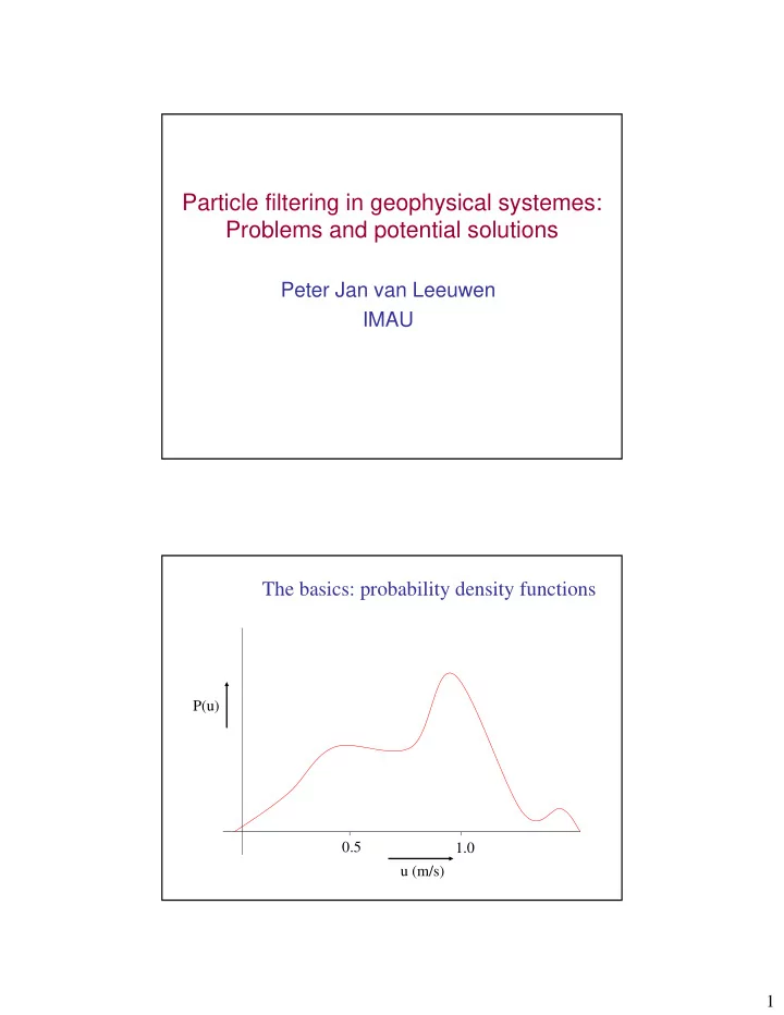
Particle filtering in geophysical systemes: Problems and potential solutions Peter Jan van Leeuwen IMAU The basics: probability density functions P(u) 0.5 1.0 u (m/s) 1
Data assimilation: general formulation NO INVERSION !!! Propagation of pdf: Ensemble methods ‘efficient’ propagation for nonlinear models 2
Model pdf’s are non-Gaussian 10 Probability density function of layer 8 thickness of first layer 6 at day 41 during 4 data-assimilation Kalman filter ? 2 Variational methods ? 0 408 412 416 420 424 428 432 436 440 444 448 452 456 Sequential Importance Sampling SIS Use ensemble with 3
Specifics of Bayes I We are interested in: Using Bayes: But also: q is the proposal density, from which it is ‘easy to draw samples’, and which might be conditioned on the new observations! Specifics of Bayes II Introduce particles drawn from q: Hence, again: But now with weights: 4
Specifics of Bayes III It is possible to use particles from the prior that have been ‘modified’ to be closer to the observations. Example: The Guided SIR Do SIR at time t2’with observations from t2. Increase observational Errors. In this case q is represented by the SIR sample from t2’. The extra weights from t2’ (in the resampled ensemble) have to be compensated for: 5
Filter degeneracy After a few updates the weights become more and more skewed: Practice: after a few updates only one member has large weight, rest has weight zero… Possible solution: - Resampling, such that all particles have equal weight again -> SIR - Integrate past times out -> MPF Sequential Importance Resampling SIR 6
SIR-results for a quasi-geostrophic ocean model around South Africa with 512 members Total variance in each layer 7
Variance-increase in non-Gaussian updates Other measure of uncertainty is ENTROPY : Filter degeneracy II: wide model pdf Observation Prior ensemble Observation Posterior ensemble EnKF Posterior ensemble SIR Observation 8
Filter degeneracy III: narrow model pdf Prior ensemble Observation Posterior ensemble EnKF Observation Observation Posterior ensemble SIR Marginal Particle Filter I The SIS updates the full joint (in time) pdf, so let’s integrate the past out -> Marginal Particle Filter. Prior: Hence: 9
Marginal Particle Filter II Use proposal density of similar form: Draw from j (i.e. run the proposal model N times with different forcing from the prior ensemble , for each member j) Calculate importance weights: And normalize them. SIR versus Marginal Particle Filter • MPF is an O(N^2) method • SIR suffers from sample noise due to resampling • Several resampling methods posible: - sample directly from weighted ensemble - residual sampling - universal sampling 10
SIR on large-scale problem: • SIR still degenerate: - weights differ too much (variance too high) - hence very small ensemble to resample from • Larger ensemble not realistic Possible solutions • Explore proposal density • Approximations in formalism • Follow solutions used in Ensemble Kalman Filter (EnKF) 11
Exploring the proposal density: Auxilary Particle Filter I (Adaptive Particle Filter) One of the reasons that the SIR fails is that the likelihood in geophysical problems is very narrow: the prior ensemble is much wider than the pdf of the observations. Hence, the majority of the particles gets very low weight. Use the observations to guide the ensemble, i.e. determine the weights of the posterior ensemble at time n-1 with respect to the new observations at time n . Auxilary Particle Filter II • Generate representation of each at i time n . ( Use e.g. the model with zero random forcing.) • Calculate weights (as normal, from likelihood) • Resample particles at time n-1 i • Run SIS (or SIR) with the new prior ensemble from time n-1 12
Approximate Particle Filters Merging Particle Filter: Generate linear combinations from prior ensemble that preserve mean and variance. Hence, the scheme is still variance minimizing (unlike EnKF and its variants..) Kernel dressing: ‘Dress’ each particle with a continuous pdf (usually a Gaussian) to obtain a global continuous pdf. Update both particles (mean of pdf’s) and covariances (using KF-like update). (Related to Gaussian mixture models) Maximum Entropy Particle Filter: Maximum Entropy Particle Filter I Without observations the pdf is the ‘background pdf’ Q. The model pdf p relaxes to this pdf in absence of observations. Q usually taken as a Gaussian mixture, with coefficients found from ‘model climatology’. When observations are present the model pdf p will be as close as possible to Q, and follows the observations as constraints. The closeness to Q is expressed as the relative entropy: 13
Maximum Entropy Particle Filter II H is maximum when p is given by: With and the lagrange multipliers, found from In which Maximum Entropy Particle Filter III • Run ensemble to observation time • Calculate η and P from the ensemble • Determine λ and Λ • Use Bayes with Gaussian statistics to update λ and Λ: • Sample new ensemble from new p 14
Costs of SIR, EnKF, MEPF • All need integration of particles • SIR analysis: O(Nnm) • EnKF analysis O(Nnm) • MEPF analysis O(Mn^2 n_max) with M number of mixtures in Q and n_max number of EOF’s of C Solution used in EnKF (Ensemble Kalman Filter) ? Local updating 15
Local updating • Reduces spurious covariances due to small ensemble size • Decouples ensemble members in different areas --> Increase of effective ensemble size • Brings ‘new blood’ in the ensemble Local SIR: use only local obs in the weights SIR Local SIR Easy to implement, but for the resampling step 16
How to do the resampling? • In SIR all particles are always balanced • In Local SIR they are not. How do we glue different particles together? Relative weight of member 1 Resampling in Local SIR • Use the pdf: • Adapt the forcing locally (Local smoother) • Use EnKF solution as ‘background field’ 17
Resampling using pdf • Start at some model point and choose randomly from weighted ensemble • Run along the grid and use this member as long as weight > 1 • When at some point x the weight < 1 choose randomly among those members that: 1 Have high weight at x 2 Resemble member at x-dx (i.e. distance smaller than standard deviation) • In this way the probabilistic features are kept! 0 2 4 6 8 10 30 30 Local smoother 28 28 26 26 24 24 Random forcing 22 22 20 20 Model trajectory 18 18 Particle 17 Particle 3 16 16 Apply weights 14 14 on forcing, 12 12 but locally !!! Particle 7 10 10 0 2 4 6 8 10 -5.5-5.4-5.3-5.2-5.1-5.0-4.9-4.8-4.7-4.6-4.5 18
Practical implementation 1 Run particles to observation time. 2 Determine local weights 3 Generate equal-weight forcing ensemble from locally weighted particles 4 Re-run the particles with this forcing ensemble 5 Either: Back to 1 OR Apply SIR with new prior weights For 3 use repeatable random field generator Use EnKF as background ensemble • Perform Local SIS • Resample such that member 1 is as close as possible to EnKF-member 1 Note: allows for use of EnKF-solution in areas when all members are far from observations 19
Conclusions • ‘Standard’ Particle Filters (SIS, SIR) do not work on large-scale problems • Maybe smart proposal pdf helps (use of Dyn. Sys. Theory?) • Maybe localization helps • Approximate Particle Filters might be needed Remarks • What do we want from particle filtering? • Mean? • Mode? • Modal information? • …. 20
. . . . . . Example 0 2 4 6 8 10 30 30 28 28 Two-layer primitive equation model of a double gyre. 26 26 24 24 Lx=2000 km, Ly = 4000 km ∆ x, ∆ y = 20 km 22 22 20 20 H1=1000 m, H2=4000 m 18 18 Wind profile 0.6 cos (y/L) 16 16 Observations 14 14 sea-surface height 12 12 ∆ x = 40 km, σ = 2 cm 10 10 0 2 4 6 8 10 Interval: 10 days (others..) -5.5-5.4-5.3-5.2-5.1-5.0-4.9-4.8-4.7-4.6-4.5 21
0 2 4 6 8 10 30 30 Statistics 28 28 26 26 24 24 Red noise random fields added to layer 22 22 thicknesses . 20 20 18 18 64 members, 16 16 80% local, 14 14 20% global 12 12 10 10 0 2 4 6 8 10 -80 -40 0 40 22
Variance reduction upper layer 2 4 6 8 2 4 6 8 28 28 28 28 Variance 26 26 26 26 Variance upper upper 24 24 24 24 layer layer 22 22 22 22 before after analysis analysis 20 20 20 20 18 18 18 18 16 16 16 16 14 14 14 14 12 12 12 12 2 4 6 8 2 4 6 8 0 50 100 0 50 100 Entropy upper layer thickness 0 0 2 2 4 4 6 6 8 8 10 10 0 0 2 2 4 4 6 6 8 8 10 10 30 30 30 30 30 30 30 30 28 28 28 28 28 28 28 28 Entropy Entropy Entropy Entropy 26 26 26 26 26 26 26 26 after after before before 24 24 24 24 24 24 24 24 analysis analysis analysis analysis at day 50 at day 50 at day 50 at day 50 22 22 22 22 22 22 22 22 20 20 20 20 20 20 20 20 18 18 18 18 18 18 18 18 16 16 16 16 16 16 16 16 14 14 14 14 14 14 14 14 12 12 12 12 12 12 12 12 10 10 10 10 10 10 10 10 0 0 2 2 4 4 6 6 8 8 10 10 0 0 2 2 4 4 6 6 8 8 10 10 0 0 1 1 2 2 3 3 4 4 0 0 1 1 2 2 3 3 4 4 23
Recommend
More recommend
Explore More Topics
Stay informed with curated content and fresh updates.
