Parameter Estimation and Model Selection of Gravitational-Wave - PowerPoint PPT Presentation
Parameter Estimation and Model Selection of Gravitational-Wave Signals Contaminated by Transient Detector Noise Glitches Jade Powell OzGrav, Swinburne University of Technology 2. Gravitational Wave Detectors 3. Detector Locations 4.
Parameter Estimation and Model Selection of Gravitational-Wave Signals Contaminated by Transient Detector Noise Glitches Jade Powell OzGrav, Swinburne University of Technology
2. Gravitational Wave Detectors
3. Detector Locations
4. Gravitational Wave Sources
5. Current Black Hole Detections 6 Binary black hole signals detected so far. Estimated distances between 340 and 1000 Mpc. One signal detected by three detectors. Image from first detection paper GW150914 (Phys- RevLett.116.061102)
6. The Neutron Star Detection GW170817 Source masses 1 . 36 − 2 . 26 M ⊙ and 0 . 86 − 1 . 36 M ⊙ Distance 40 Mpc
7. Parameter Estimation Measuring parameters of a source is essential for astrophysics with gravitational wave detections. With GW detectors we can measure the chirp mass, spin, eccentricity, distance, and sky position. Chirp mass is given by M = ( m 1 m 2 ) 3 / 5 / ( m 1 + m 2 ) 1 / 5
8. Astrophysics with Source Parameters Constrain the mass distribution of black hole binaries. Distinguish between different black hole formation channels. Attempt to constrain parameters in binary evolution using population synthesis models. Measure the evolution of merger rate / mass distribution with redshift.
9. Bayesian Model Selection
10. Parameter Estimation To calculate the evidence for each model we integrate the likelihood multiplied by the prior over all possible parameter values θ � p ( D | M ) = p ( θ | M ) p ( D | θ, M ) d θ. (1) θ The evidence integral is difficult for a large number of parameters. This problem is solved using nested sampling.
11. Nested Sampling First the likelihood is calculated for selected points distributed over the entire prior. The point with the smallest likelihood and largest prior mass is selected and becomes the limiting values. A new point is generated inside the new limits. This is repeated so that it iterates inwards in prior mass and upwards in likelihood until the highest value is found. Produces Bayes factors and posterior distributions on the signal parameters.
12. Burst Sources For a burst source we don’t know exactly what a signal should look like. We use sine Gaussian’s as a signal model. They are defined as, h x ( t ) = h 0 sin(2 π ft ) exp( − t 2 /τ 2 ) (2) h + ( t ) = h 0 cos(2 π ft ) exp( − t 2 /τ 2 ) (3) √ where τ = Q / 2 π f , f is the frequency, Q is the quality factor, t is time of the signal and h 0 = hrss / √ τ , where hrss is the root sum squared amplitude of the signal. Produces posterior distributions on hrss, Q, f, and sky position.
13. Glitches Glitches are short duration excess power noise created by the detector or the environment. The detectors have 1000’s of auxiliary channels of data from monitors around the detector. Some glitches don’t show up in any monitors making it difficult to determine their origin. They limit the sensitivity of gravitational wave searches.
14. Signals with glitches 10 6 glitches above SNR 6 were observed in 51.5 days of O1. GW170817 had a large glitch in L1. High probability that as detections increase, more will occur at the same time as a glitch.
15. Glitch Removal For GW170817 we already know what we expected the signal to look like. The glitch was very loud and easy to identify as being a glitch. It was removed by gating and subtracting the reconstructed waveform. The glitch is short duration compared to the signal, which means some signal is still left over after gating. It might not be so easy next time!
16. This Analysis We inject three different types of gravitational wave signals on top of three different types of glitches. We measure the parameters of the signals at different signal to noise ratios and offsets in time between the signal and glitches. What happens if the glitch is not obvious because it does not occur in auxiliary channels and the exact shape of the signal waveform is unknown? We determine the effects of glitches that can’t be gated. We investigate if the effects of glitches is worse when there is a mis-match between signal and template.
17. The Glitches Three types of O1 glitches are used that occur in L1 at the same time as good quality H1 data. Figure: Images taken from Gravity Spy.
18. The Signals 3 Binary black hole 2 1 0 1 We measure parameters of all signals 2 injected near glitches with time offsets 3 0.10 0.08 0.06 0.04 0.02 0.00 0.02 Time(s) of 0.0 s, 0.1 s and 0.2 s. 1.0 Supernova IMRPhenomPv2 signal model is used 0.5 for the CBC signals. 0.0 A sine Gaussian signal model is used 0.5 for the sine Gaussian signals. 0.00 0.25 0.50 0.75 1.00 1.25 Time(s) A sine Gaussian model is used for the 6 Sine Gaussian 4 supernova signals to determine if 2 effects are worse when there is a 0 mis-match between signal and model. 2 4 6 0.04 0.02 0.00 0.02 0.04 Time(s)
19. BBH Bayes Factors 500 500 scattering scattering blip blip whistle whistle 400 400 offset 0.0s offset 0.1s 300 300 log B log B 200 200 100 100 0 0 0 5 10 15 20 25 30 0 5 10 15 20 25 30 Signal SNR Signal SNR 500 25 scattering blip whistle 400 20 offset 0.2s Glitch SNR 300 15 log B 200 10 100 5 scattering blip whistle 0 0 0 5 10 15 20 25 30 0 5 10 15 20 25 30 Signal SNR Signal SNR
20. BBH Example Posteriors true value offset 0.0s 2500 offset 0.1s offset 0.2s 2000 1500 1000 500 0 17.5 20.0 22.5 25.0 27.5 30.0 32.5 Chirp mass ( M ) true value 3000 offset 0.0s offset 0.1s 2500 offset 0.2s 2000 1500 1000 500 0 0 200 400 600 800 1000 1200 1400 Distance (Mpc)
21. BBH Chirp Mass Summary 30 scattering 30 scattering blip blip Posterior width ( M ) Posterior width ( M ) whistle whistle 25 25 offset 0.0s offset 0.1s 20 20 15 15 10 10 5 5 0 0 20 15 10 5 0 5 10 15 20 20 15 10 5 0 5 10 15 20 true ( M ) true ( M ) rec rec 30 scattering blip Posterior width ( M ) whistle 25 offset 0.2s 20 15 10 5 0 20 15 10 5 0 5 10 15 20 true ( M ) rec
22. BBH Distance Summary 3500 3500 scattering scattering blip blip Posterior width (Mpc) Posterior width (Mpc) 3000 3000 whistle whistle 2500 offset 0.0s 2500 offset 0.1s 2000 2000 1500 1500 1000 1000 500 500 0 0 500 0 500 1000 1500 500 0 500 1000 1500 Dist true ( Mpc ) Dist true ( Mpc ) Dist rec Dist rec 3500 scattering blip Posterior width (Mpc) 3000 whistle 2500 offset 0.2s 2000 1500 1000 500 0 500 0 500 1000 1500 Dist true ( Mpc ) Dist rec
23. Sine Gaussian Bayes Factors 600 600 scattering scattering blip blip 500 500 whistle whistle offset 0.0s offset 0.1s 400 400 log B log B 300 300 200 200 100 100 0 0 0 5 10 15 20 25 30 35 0 5 10 15 20 25 30 35 Signal SNR Signal SNR 600 25 scattering blip 500 whistle 20 offset 0.2s 400 Glitch SNR 15 log B 300 10 200 5 scattering 100 blip whistle 0 0 0 5 10 15 20 25 30 35 0 5 10 15 20 25 30 Signal SNR Signal SNR
24. Sine Gaussian Example Posteriors 1600 true value 1400 offset 0.0s offset 0.1s 1200 offset 0.2s 1000 800 600 400 200 0 160 180 200 220 240 260 280 300 320 Frequency (Hz) 2000 true value offset 0.0s 1750 offset 0.1s offset 0.2s 1500 1250 1000 750 500 250 0 52 51 50 49 48 log hrss
25. Sine Gaussian Frequency Summary 200 200 scattering scattering 175 blip 175 blip Posterior width (Hz) Posterior width (Hz) whistle whistle 150 150 offset 0.0s offset 0.1s 125 125 100 100 75 75 50 50 25 25 0 0 250 0 250 500 750 1000 1250 1500 1750 250 0 250 500 750 1000 1250 1500 1750 f true ( Hz ) f true ( Hz ) f rec f rec 200 scattering 175 blip Posterior width (Hz) whistle 150 offset 0.2s 125 100 75 50 25 0 250 0 250 500 750 1000 1250 1500 1750 f true ( Hz ) f rec
26. Sine Gaussian Log Hrss Summary 1.8 1.8 scattering scattering 1.6 1.6 blip blip whistle whistle 1.4 1.4 Posterior width Posterior width offset 0.0s offset 0.1s 1.2 1.2 1.0 1.0 0.8 0.8 0.6 0.6 0.4 0.4 0.2 0.2 0.0 0.0 3 2 1 0 1 2 3 3 2 1 0 1 2 3 loghrss rec loghrss true loghrss rec loghrss true 1.8 scattering 1.6 blip whistle 1.4 Posterior width offset 0.2s 1.2 1.0 0.8 0.6 0.4 0.2 0.0 3 2 1 0 1 2 3 loghrss rec loghrss true
27. Supernova Bayes Factors 400 400 scattering scattering 350 blip 350 blip whistle whistle 300 300 offset 0.0s offset 0.1s 250 250 log B log B 200 200 150 150 100 100 50 50 0 0 0 5 10 15 20 25 30 35 0 5 10 15 20 25 30 35 Signal SNR Signal SNR 400 25 scattering 350 blip whistle 20 300 offset 0.2s Glitch SNR 250 15 log B 200 10 150 100 5 scattering blip 50 whistle 0 0 0 5 10 15 20 25 30 35 0 5 10 15 20 25 30 Signal SNR Signal SNR
28. Supernova Example Posteriors 3000 true value offset 0.0s 2500 offset 0.1s offset 0.2s 2000 1500 1000 500 0 0.0 0.1 0.2 0.3 0.4 0.5 0.6 0.7 Duration (s) 2000 true value offset 0.0s 1750 offset 0.1s offset 0.2s 1500 1250 1000 750 500 250 0 52 51 50 49 48 log hrss
Recommend
More recommend
Explore More Topics
Stay informed with curated content and fresh updates.
