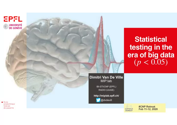
( p < 0.05) Dimitri Van De Ville MIP:lab IBI-STI/CNP (EPFL) - - PowerPoint PPT Presentation

Statistical testing in the era of big data


(p < 0.05)

Dimitri Van De Ville


MIP:lab

IBI-STI/CNP (EPFL) 
 RADIO (UniGE)


http://miplab.epfl.ch/ @dvdevill #CNP Retreat
 Feb 11-12, 2020

Dimitri Van De Ville CNP Retreat 2020 — Stats Workshop 2

Panic

Dimitri Van De Ville CNP Retreat 2020 — Stats Workshop 3

Big Data

Dimitri Van De Ville CNP Retreat 2020 — Stats Workshop 4

Paradox?

Mount
 Big
 Data

p<0.05

Is big data destroying 
 p-values?

Dimitri Van De Ville CNP Retreat 2020 — Stats Workshop

▪ Contradictory tendencies ▪ Many (emotive) reports about p-value crisis ▪ Reviewers even more picky on statistical significance ▪ Sufficient power, multiple comparisons, replication,… ▪ Adage: Never enough data ▪ Big data has arrived, and will become bigger ▪ Is classical hypothesis testing doomed?


Should we all go into Bayesian statistics?
 Machine-learning approaches will be the only solution?

▪ Here, revisit the basic statistical hypothesis testing ▪ to understand the core issue ▪ to solve it within the conventional framework

Roadmap of the workshop

5

Dimitri Van De Ville CNP Retreat 2020 — Stats Workshop

▪ Consider

samples modeled to reflect a true effect with a random Gaussian* deviation : ,

▪ Estimator of is average ▪ Estimator of uncertainty on is standard deviation ▪ We define ▪ Question: is there evidence from the data that the underlying

N μ 𝒪(0,σ2) xn = μ + en n = 1,…, N μ ̂ μ ̂ μ ̂ σ t = ̂ μ ̂ σ N μ ≠ 0

One-sample t-test in a nutshell

6

* Popularity of Gaussian hypothesis? Central limit theorem!

Dimitri Van De Ville CNP Retreat 2020 — Stats Workshop

▪ Null hypothesis

: no effect,

▪ (Implicit) alternative hypothesis

:

▪ Under the null, follows a known distribution 


(Student t-distribution with degrees of freedom)

▪

• value is probability to mistakenly reject

:

▪ Result is considered significant if <0.05

ℋ0 μ = 0 ℋ1 μ ≠ 0 t

N − 1

p ℋ0 p = P(|t| > T|ℋ0) p

One-sample t-test in a nutshell

7

“If one in twenty does not seem high enough odds, we may, if we prefer it, draw the line at one in fifty or one in a hundred. Personally, the writer prefers to set a low standard of significance at the 5 per cent point, and ignore entirely all results which fails to reach this level.”

— R.A. Fisher, “The arrangement of field experiments”. Journal of the Ministry of Agriculture of Great Britain. 33:503-513, 1926

Dimitri Van De Ville CNP Retreat 2020 — Stats Workshop

▪ Thus, -value indicates probability of false positive (FP) ▪ Typically, no explicit

:

▪ No control on false negatives; i.e., ▪ One can only control specificity (1-FP rate), not sensitivity (1-FN rate) ▪ No proof of no effect because no point of comparison

p ℋ1 P(|t| ≤ T|ℋ1 not true)

One-sample t-test in a nutshell

8

Dimitri Van De Ville CNP Retreat 2020 — Stats Workshop

▪ Any true effect

can become significant for sufficiently large

▪ “[

] must be big enough that an effect of such magnitude as to be of scientific significance will also be statistically significant. It is just as important, however, that the study not be too big, where an effect of little scientific importance is nevertheless statistically detectable”

▪ As

increases, discriminability, as measured by classification accuracy, of individual samples becomes very small

▪ As

increases, consistency, as measured by population prevalence, of the effect becomes very small

μ0 ≠ 0 N N N N

Fallacy of statistical testing

9

μ0 σ N > T N > T2 σ2 μ2

[Lenth, 2001]

Dimitri Van De Ville CNP Retreat 2020 — Stats Workshop

▪ Bottomline: -values are relevant if effect size is non-trivial! ▪ Standardized effect size: Cohen’s

; ; 
 
 


▪ “… one should be cautious that extremely large studies may be more likely to

find a formally statistical significant difference for a trivial effect that is not really meaningfully different from the null.” (Ioannidis, 2005)

p d = t/ N R2 = μ2/(μ2 + σ2) ρ = R2

Effect size

10

[Friston, NeuroImage, 2012]

Effect size Cohen’s d Coefficient of determination R2 Correlation Classification accuracy Population prevalence Large

~1 ~1/2=0.50 ~0.71 ~70% ~50%

Medium

~1/2=0.50 ~1/5=0.20 ~0.45 ~60% ~20%

Small

~1/4=0.25 ~1/17=0.06 ~0.24 ~55% ~6%

Trivial

~1/8=0.13 ~1/65=0.02 ~0.12 ~52.5% ~1%

None

50% 0%

Dimitri Van De Ville CNP Retreat 2020 — Stats Workshop

▪ Consider now fixed specificity

, then we have


α = 0.05 α = ∫

∞ u(α)

T(t; N − 1)dt

Sample size and sensitivity

11

[Friston, NeuroImage, 2012]

α T|ℋ0

Dimitri Van De Ville CNP Retreat 2020 — Stats Workshop

▪ Consider now fixed specificity

, then we have


▪ Under the assumption of a true effect size , we can compute sensitivity as



 where is the non-central
 t-distribution with degrees of 
 freedom and non-centrality 
 parameter

▪ Sensitivity depends on sample 


size ( ) and effect size ( )

α = 0.05 α = ∫

∞ u(α)

T(t; N − 1)dt d 1 − β(d) = ∫

∞ u(α)

T(t; N − 1,d N)dt T(t; K, δ) K δ N d

Sample size and sensitivity

12

[Friston, NeuroImage, 2012]

α 1 − β T|ℋ0 T|ℋ1

Dimitri Van De Ville CNP Retreat 2020 — Stats Workshop

▪ Sensitivity depends on sample size (

) and effect size ( )

▪ Significant effect with small sample size


is likely to be caused by large effect
 size!

▪ If you are criticized in this way:



 “The fact that we have demonstrated a 
 significant result in a relatively under-
 powered study suggests that the effect 
 size is large. This means, quantitatively, 


• ur result is stronger than if we had 


used a larger sample-size.”
 
 = conflation of significance and power

N d

Under-powered?

13

[Friston, NeuroImage, 2012]

1 − β(d)

50 % 0 % 100 %

Dimitri Van De Ville CNP Retreat 2020 — Stats Workshop

▪ Sensitivity depends on sample size (

) and effect size ( )

▪ Sensitivity to trivial effect sizes 


increases with sample size!

▪ Ultimately, with very large sample 


sizes, sensitivity will reach 100%
 for every non-null effect size

▪ Explains a lot about the crisis! ▪ More is not better

N d

10 20 30 40 50 60 70 80 90 100

sample size

0.1 0.2 0.3 0.4 0.5 0.6 0.7 0.8 0.9 1

sensitivity

Over-powered?

14

[Friston, NeuroImage, 2012]

Dimitri Van De Ville CNP Retreat 2020 — Stats Workshop

10 20 30 40 50 60 70 80 90 100

sample size

• 1
• 0.9
• 0.8
• 0.7
• 0.6
• 0.5
• 0.4
• 0.3
• 0.2
• 0.1

loss

10 20 30 40 50 60 70 80 90 100

sample size

• 1
• 0.9
• 0.8
• 0.7
• 0.6
• 0.5
• 0.4
• 0.3
• 0.2
• 0.1

loss

▪ Let us define a simple loss function : ▪ Cost

for detecting trivial effect size of [bad]

▪ Cost

for detecting large effect size of [good]

▪ Expected loss:


▪ Optimal sample size at minimal loss ▪ Does not increase dramatically even


if significance needs to be (much)
 stronger (e.g., due to multiple 
 comparisons)

l +1 1/8 −1 1 l = (1 − β(1/8)) − (1 − β(1)) = β(1) − β(1/8)

Loss-function analysis

15

Dimitri Van De Ville CNP Retreat 2020 — Stats Workshop 10 20 30 40 50 60 70 80 90 100

sample size

0.1 0.2 0.3 0.4 0.5 0.6 0.7 0.8 0.9 1

sensitivity

▪ Inference is based on controlling FP rate under

, which translates in a flat sensitivity at for no effect:

▪ specificity = 


sensitivity to null effects

▪ So let us suppress sensitivity to 


trivial effects instead!
 
 where this time we use



 with

ℋ0 α

1 − β(d) = ∫

∞ u(α)

T(t; N − 1,d N)dt α(d′) = ∫

∞ u(α)

T(t; N − 1,d′ N)dt d′ = 1/8

Protected inference

16

[Friston, NeuroImage, 2012]

10 20 30 40 50 60 70 80 90 100

sample size

0.1 0.2 0.3 0.4 0.5 0.6 0.7 0.8 0.9 1

sensitivity

specificity

Dimitri Van De Ville CNP Retreat 2020 — Stats Workshop

▪ Protection fixes

and thus increasing becomes harmless

▪ Concretely, threshold to be applied to -values is penalized

β(1/8) = 0.05 N t

Protected inference

17 10 20 30 40 50 60 70 80 90 100

sample size

• 1
• 0.9
• 0.8
• 0.7
• 0.6
• 0.5
• 0.4
• 0.3
• 0.2
• 0.1

loss

10 20 30 40 50 60 70 80 90 100

sample size

1 2 3 4 5 6 7 8 9 10

T threshold no protection protection [Friston, NeuroImage, 2012]

Dimitri Van De Ville CNP Retreat 2020 — Stats Workshop

▪ Consider

samples modeled to reflect a true effect with a random deviation of unknown, but symmetric distribution: ,

▪ Estimator of is average (could also be median etc) ▪ Null hypothesis

: no effect,

▪ In that case, we can randomly flip or permute the signs of

and recompute our measure of interest under the null as ,

▪ If

• r

, then is rejected with

▪ Use

randomizations to be able to assess 0.05 significance

▪ Less assumptions about distribution, but essentially same problem that

trivial effects will be picked up as increases

N μ xn = μ + en n = 1,…, N μ ̂ μ ℋ0 μ = 0 xn ̂ μ(0)

k

k = 1,…, K ̂ μ > max ̂ μ(0)

k

̂ μ < min ̂ μ(0)

k

ℋ0 p = 2/(K + 1) K = 39 N

A note on non-parametric testing

18

Dimitri Van De Ville CNP Retreat 2020 — Stats Workshop

▪ Inferential statistics; e.g., presence of treatment effect ▪ In-sample effect size is about data at hand ▪ In-sample effect size overestimates true effect size because some large

test statistics can also be obtained by chance

▪ Estimation; e.g., predicting treatment effect ▪ Out-of-sample effect size 


is an unbiased estimate 


• f true effect size

▪ However, test is less


efficient

▪ Le beurre et 


l’argent du beurre

Bias-variance trade-off of effect size

19

[Friston, NeuroImage, 2012]

Dimitri Van De Ville CNP Retreat 2020 — Stats Workshop

▪ More data allows you to do more things ▪ Terminology becomes important!

Reproducible science

20

Dimitri Van De Ville CNP Retreat 2020 — Stats Workshop

And some resources

21

https://www.nature.com/collections/qghhqm/pointsofsignificance

Dimitri Van De Ville CNP Retreat 2020 — Stats Workshop

▪ The nine circles of scientific hell

Good luck… and stay out of hell!

22

[Neuroskeptic,Perspectives on Psychological Science, 2012]

I Limbo II Lust III Gluttony IV Greed V Anger VI Heresy VII Violence VIII Fraud IX Treachery

@Neuro_Skeptic

I Limbo II Overselling III Post-Hoc Storytelling IV P-Value Fishing V Creative Outliers VI Plagiarism VII Non-Publication VIII Partial Publication IX Inventing Data