Outline Scale-Free Networks Networks Scale-Free Networks - PowerPoint PPT Presentation
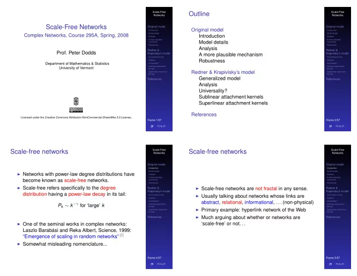
Scale-Free Outline Scale-Free Networks Networks Scale-Free Networks Original model Original model Original model Introduction Introduction Model details Model details Complex Networks, Course 295A, Spring, 2008 Introduction Analysis
Scale-Free Outline Scale-Free Networks Networks Scale-Free Networks Original model Original model Original model Introduction Introduction Model details Model details Complex Networks, Course 295A, Spring, 2008 Introduction Analysis Analysis A more plausible A more plausible Model details mechanism mechanism Robustness Robustness Analysis Redner & Redner & Prof. Peter Dodds Krapivisky’s model Krapivisky’s model A more plausible mechanism Generalized model Generalized model Robustness Analysis Analysis Department of Mathematics & Statistics Universality? Universality? Sublinear attachment Sublinear attachment University of Vermont kernels kernels Redner & Krapivisky’s model Superlinear attachment Superlinear attachment kernels kernels Generalized model References References Analysis Universality? Sublinear attachment kernels Superlinear attachment kernels References Licensed under the Creative Commons Attribution-NonCommercial-ShareAlike 3.0 License . Frame 1/57 Frame 2/57 Scale-free networks Scale-Free Scale-free networks Scale-Free Networks Networks Original model Original model Introduction Introduction Model details Model details ◮ Networks with power-law degree distributions have Analysis Analysis A more plausible A more plausible become known as scale-free networks. mechanism mechanism Robustness Robustness ◮ Scale-free refers specifically to the degree ◮ Scale-free networks are not fractal in any sense. Redner & Redner & Krapivisky’s model Krapivisky’s model distribution having a power-law decay in its tail: ◮ Usually talking about networks whose links are Generalized model Generalized model Analysis Analysis Universality? abstract, relational, informational, . . . (non-physical) Universality? P k ∼ k − γ for ‘large’ k Sublinear attachment Sublinear attachment kernels kernels ◮ Primary example: hyperlink network of the Web Superlinear attachment Superlinear attachment kernels kernels ◮ Much arguing about whether or networks are References References ◮ One of the seminal works in complex networks: ‘scale-free’ or not. . . Laszlo Barabási and Reka Albert, Science, 1999: “Emergence of scaling in random networks” [2] ◮ Somewhat misleading nomenclature... Frame 4/57 Frame 5/57
Random networks: largest components Scale-Free Scale-free networks Scale-Free Networks Networks Original model Original model Introduction Introduction Model details Model details Analysis Analysis The big deal: A more plausible A more plausible mechanism mechanism Robustness Robustness ◮ We move beyond describing of networks to finding Redner & Redner & Krapivisky’s model Krapivisky’s model mechanisms for why certain networks are the way Generalized model Generalized model Analysis Analysis they are. γ = 2.5 γ = 2.5 γ = 2.5 γ = 2.5 Universality? Universality? � k � = 1.8 � k � = 2.05333 � k � = 1.66667 � k � = 1.92 Sublinear attachment Sublinear attachment kernels kernels Superlinear attachment Superlinear attachment kernels kernels A big deal for scale-free networks: References References ◮ How does the exponent γ depend on the mechanism? ◮ Do the mechanism details matter? γ = 2.5 γ = 2.5 γ = 2.5 γ = 2.5 � k � = 1.6 � k � = 1.50667 � k � = 1.62667 � k � = 1.8 Frame 6/57 Frame 7/57 Heritage Scale-Free BA model Scale-Free Networks Networks Original model Original model Introduction Introduction Work that presaged scale-free networks Model details Model details ◮ Barabási-Albert model = BA model. Analysis Analysis A more plausible A more plausible ◮ 1924: G. Udny Yule [9] : mechanism ◮ Key ingredients: mechanism Robustness Robustness # Species per Genus Growth and Preferential Attachment (PA). Redner & Redner & Krapivisky’s model Krapivisky’s model ◮ 1926: Lotka [4] : ◮ Step 1: start with m 0 disconnected nodes. Generalized model Generalized model Analysis Analysis # Scientific papers per author ◮ Step 2: Universality? Universality? Sublinear attachment Sublinear attachment kernels kernels ◮ 1953: Mandelbrot [5] ): 1. Growth—a new node appears at each time step Superlinear attachment Superlinear attachment kernels kernels t = 0 , 1 , 2 , . . . . Zipf’s law for word frequency through optimization References References 2. Each new node makes m links to nodes already ◮ 1955: Herbert Simon [8, 10] : present. Zipf’s law, city size, income, publications, and 3. Preferential attachment—Probability of connecting to species per genus i th node is ∝ k i . ◮ 1965/1976: Derek de Solla Price [6, 7] : ◮ In essence, we have a rich-gets-richer scheme. Network of Scientific Citations Frame 8/57 Frame 10/57
BA model Scale-Free Approximate analysis Scale-Free Networks Networks ◮ When ( N + 1 ) th node is added, the expected Original model Original model ◮ Definition: A k is the attachment kernel for a node Introduction Introduction increase in the degree of node i is Model details Model details Analysis Analysis with degree k . A more plausible A more plausible mechanism k i , N mechanism ◮ For the original model: Robustness Robustness E ( k i , N + 1 − k i , N ) ≃ m . � N ( t ) Redner & Redner & j = 1 k j ( t ) Krapivisky’s model Krapivisky’s model A k = k Generalized model Generalized model Analysis Analysis ◮ Assumes probability of being connected to is small. Universality? Universality? ◮ Definition: P attach ( k , t ) is the attachment probability. Sublinear attachment Sublinear attachment kernels kernels ◮ Dispense with Expectation by assuming (hoping) that Superlinear attachment Superlinear attachment ◮ For the original model: kernels kernels over longer time frames, degree growth will be References References smooth and stable. k i ( t ) k i ( t ) P attach ( node i , t ) = = ◮ Approximate k i , N + 1 − k i , N with d d t k i , t : � N ( t ) � k max ( t ) j = 1 k j ( t ) k = m kN k ( t ) d k i ( t ) d t k i , t = m where N ( t ) = m 0 + t is # nodes at time t � N ( t ) j = 1 k j ( t ) and N k ( t ) is # degree k nodes at time t . Frame 12/57 Frame 13/57 where t = N ( t ) − m 0 . Approximate analysis Scale-Free Approximate analysis Scale-Free Networks Networks ◮ Deal with denominator: each added node brings m Original model Original model new edges. Introduction Introduction Model details Model details ◮ Know i th node appears at time N ( t ) Analysis Analysis A more plausible A more plausible � k j ( t ) = 2 tm ∴ mechanism � i − m 0 mechanism Robustness Robustness for i > m 0 j = 1 t i , start = Redner & Redner & 0 for i ≤ m 0 Krapivisky’s model Krapivisky’s model Generalized model Generalized model ◮ The node degree equation now simplifies: Analysis Analysis ◮ So for i > m 0 (exclude initial nodes), we must have Universality? Universality? Sublinear attachment Sublinear attachment kernels kernels d k i ( t ) = mk i ( t ) 2 mt = 1 Superlinear attachment Superlinear attachment d t k i , t = m 2 t k i ( t ) � 1 / 2 kernels kernels � t � N ( t ) j = 1 k j ( t ) k i ( t ) = m for t ≥ t i , start . References References t i , start ◮ All node degrees grow as t 1 / 2 but later nodes have ◮ Rearrange and solve: larger t i , start which flattens out growth curve. d k i ( t ) k i ( t ) = d t 2 t ⇒ k i ( t ) = c i t 1 / 2 . ◮ Early nodes do best (First-mover advantage). Frame 14/57 Frame 15/57 ◮ Next find c i . . .
Recommend
More recommend
Explore More Topics
Stay informed with curated content and fresh updates.
