Marcel Dettling Institute for Data Analysis and Process Design - PowerPoint PPT Presentation
Applied Time Series Analysis FS 2011 Week 05 Marcel Dettling Institute for Data Analysis and Process Design Zurich University of Applied Sciences marcel.dettling@zhaw.ch http://stat.ethz.ch/~dettling ETH Zrich, March 21, 2011 Marcel
Applied Time Series Analysis FS 2011 – Week 05 Marcel Dettling Institute for Data Analysis and Process Design Zurich University of Applied Sciences marcel.dettling@zhaw.ch http://stat.ethz.ch/~dettling ETH Zürich, March 21, 2011 Marcel Dettling, Zurich University of Applied Sciences 1
Applied Time Series Analysis FS 2011 – Week 05 Basic Idea for AR-Models We have a time series where, resp. we model a time series such that the random variable depends on a linear combination of X 1 ,..., X the preceding ones , plus a „completely independent“ t t p term called innovation . E t X X ... X E t 1 t 1 p t p t p is called the order of the AR-model. We write AR(p). Note that there are some restrictions to . E t Marcel Dettling, Zurich University of Applied Sciences 2
Applied Time Series Analysis FS 2011 – Week 05 AR(1)-Model The simplest model is the AR(1)-model X X E t 1 t 1 t where 2 Var E ( ) is i.i.d with and E E E [ ] 0 t E t t Under these conditions, is a white noise process, and we E t additionally require causality , i.e. being an innovation : E t X , s t E is independent of s t Marcel Dettling, Zurich University of Applied Sciences 3
Applied Time Series Analysis FS 2011 – Week 05 Causality Note that causality is an important property that, despite the fact that it‘s missing in much of the literature, is necessary in the context of AR-modeling: E is an innovation process all are independent E t t All are independent E is an innovation E t t Marcel Dettling, Zurich University of Applied Sciences 4
Applied Time Series Analysis FS 2011 – Week 05 Simulated AR(1)-Series Simulated AR(1)-Series: alpha_1=0.7 4 3 2 1 ts.sim 0 -1 -2 -3 0 50 100 150 200 Time Marcel Dettling, Zurich University of Applied Sciences 5
Applied Time Series Analysis FS 2011 – Week 05 Simulated AR(1)-Series Simulated AR(1)-Series: alpha_1=-0.7 3 2 1 ts.sim 0 -1 -2 -3 -4 0 50 100 150 200 Time Marcel Dettling, Zurich University of Applied Sciences 6
Applied Time Series Analysis FS 2011 – Week 05 Simulated AR(1)-Series Simulated AR(1)-Series: alpha_1=1 -275 -280 ts.sim -285 -290 0 50 100 150 200 Time Marcel Dettling, Zurich University of Applied Sciences 7
Applied Time Series Analysis FS 2011 – Week 05 Moments of the AR(1)-Process Some calculations with the moments of the AR(1)-process give insight into stationarity and causality Proof: See blackboard… Marcel Dettling, Zurich University of Applied Sciences 8
Applied Time Series Analysis FS 2011 – Week 05 Theoretical vs. Estimated ACF True ACF of AR(1)-process with alpha_1=0.7 1.0 0.8 0.6 ACF 0.4 0.2 0.0 0 50 100 150 200 lag Estimated ACF from an AR(1)-series with alpha_1=0.7 1.0 0.6 ACF 0.2 -0.2 0 50 100 150 200 Marcel Dettling, Zurich University of Applied Sciences 9 Lag
Applied Time Series Analysis FS 2011 – Week 05 Theoretical vs. Estimated ACF True ACF of AR(1)-process with alpha_1=-0.7 1.0 0.5 ACF 0.0 -0.5 0 50 100 150 200 lag Estimated ACF from an AR(1)-series with alpha_1=-0.7 1.0 0.5 ACF 0.0 -0.5 0 50 100 150 200 Marcel Dettling, Zurich University of Applied Sciences 10 Lag
Applied Time Series Analysis FS 2011 – Week 05 AR(p)-Model We here introduce the AR(p)-model X X ... X E t 1 t 1 p t p t where again 2 Var E ( ) is i.i.d with and E E E [ ] 0 t E t t Under these conditions, is a white noise process, and we E t additionally require causality , i.e. being an innovation : E t X , s t E is independent of s t Marcel Dettling, Zurich University of Applied Sciences 11
Applied Time Series Analysis FS 2011 – Week 05 Mean of AR(p)-Processes As for AR(1)-processes, we also have that: ( X ) E X [ ] 0 is from a stationary AR(p) => t t T t E X [ ] 0 Thus: If we observe a time series with , it cannot t be, due to the above property, generated by an AR(p)- process But: In practice, we can always de-“mean“ (i.e. center) a stationary series and fit an AR(p) model to it. Marcel Dettling, Zurich University of Applied Sciences 12
Applied Time Series Analysis FS 2011 – Week 05 Yule-Walker-Equations On the blackboard… We observe that there exists a linear equation system built up from the AR(p)-coefficients and the ACF-coefficients of up to lag p. These are called Yule-Walker-Equations. We can use these equations for fitting an AR(p)-model: 1) Estimate the ACF from a time series 2) Plug-in the estimates into the Yule-Walker-Equations 3) The solution are the AR(p)-coefficients Marcel Dettling, Zurich University of Applied Sciences 13
Applied Time Series Analysis FS 2011 – Week 05 Stationarity of AR(p)-Processes We need: E X [ ] 0 1) t ( ,..., ) 2) Conditions on 1 p All (complex) roots of the characteristic polynom 2 p 1 z z z 0 1 2 p need to lie outside of the unit circle. This can be checked with R-function polyroot() Marcel Dettling, Zurich University of Applied Sciences 14
Applied Time Series Analysis FS 2011 – Week 05 A Non-Stationary AR(2)-Process 1 1 X X X E is not stationary… 1 2 t t t t 2 2 Non-Stationary AR(2) 5 0 -5 -10 0 100 200 300 400 Marcel Dettling, Zurich University of Applied Sciences 15 Time
Applied Time Series Analysis FS 2011 – Week 05 Fitting AR(p)-Models This involves 3 crucial steps: 1) Is an AR(p) suitable, and what is p? - will be based on ACF/PACF-Analysis 2) Estimation of the AR(p)-coefficients - Regression approach - Yule-Walker-Equations - and more (MLE, Burg-Algorithm) 3) Residual Analysis - to be discussed Marcel Dettling, Zurich University of Applied Sciences 16
Applied Time Series Analysis FS 2011 – Week 05 AR-Modelling 1 2 3 Identification Parameter Model of the Order p Estimation Diagnostics - ACF/PACF - Regression - Residual Analysis - AIC/BIC - Yule-Walker - Simulation - MLE - Burg Marcel Dettling, Zurich University of Applied Sciences 17
Applied Time Series Analysis FS 2011 – Week 05 Is an AR(p) suitable, and what is p? - For all AR(p)-models, the ACF decays exponentially quickly, or is an exponentially damped sinusoid. - For all AR(p)-models, the PACF is equal to zero for all lags k>p. If what we observe is fundamentally different from the above, it is unlikely that the series was generated from an AR(p)-process. We thus need other models, maybe more sophisticated ones. Remember that the sample ACF has a few peculiarities and is tricky to interpret!!! Marcel Dettling, Zurich University of Applied Sciences 18
Applied Time Series Analysis FS 2011 – Week 05 Model Order for sqrt(purses) 6 5 series 4 3 2 1968 1969 1970 1971 1972 1973 Time 1.0 part. Autokorr Auto-Korr. 0.2 0.4 -0.2 -0.2 0 5 10 15 1 5 10 15 Lag k Lag k Marcel Dettling, Zurich University of Applied Sciences 19
Applied Time Series Analysis FS 2011 – Week 05 Model Order for log(lynx) 9 8 7 series 6 5 4 1820 1840 1860 1880 1900 1920 Time part. Autokorr 0.5 Auto-Korr. 0.5 -0.5 -0.5 0 5 10 15 20 1 5 10 15 20 Lag k Lag k Marcel Dettling, Zurich University of Applied Sciences 20
Applied Time Series Analysis FS 2011 – Week 05 Basic Idea for Parameter Estimation We consider the stationary AR(p) ( X ) ( X ) ... ( X ) E t 1 t 1 p t p t where we need to estimate 1 ,..., model parameters p 2 innovation variance E general mean Marcel Dettling, Zurich University of Applied Sciences 21
Applied Time Series Analysis FS 2011 – Week 05 Approach 1: Regression Response variable: , t = 1,…,n X t Explanatory variables: , t = 2,…,n X 1 t , t = 3,…,n X t 2 … X , t = p+1,…,n t p We can now use the regular LS framework. The coefficient estimates then are the estimates for . Moreover, we have 1 ,..., p ˆ n p 1 2 2 0 and ˆ r E i n 2 p 1 ˆ ˆ ˆ 1 ... i 1 1 2 p Marcel Dettling, Zurich University of Applied Sciences 22
Applied Time Series Analysis FS 2011 – Week 05 Approach 1: Regression Preparing the design matrix > d.Psqrt <- sqrt(Purses) > d.Psqrt.mat <- ts.union(Y=d.Psqrt,X1=lag(d.Psqrt,-1),X2=lag(d.Psqrt,-2)) > d.Psqrt.mat[1:5,] Y X1 X2 [1,] 3.162 NA NA [2,] 3.873 3.162 NA [3,] 3.162 3.873 3.162 [4,] 3.162 3.162 3.873 [5,] 3.464 3.162 3.162 Marcel Dettling, Zurich University of Applied Sciences 23
Recommend
More recommend
Explore More Topics
Stay informed with curated content and fresh updates.
