n-grams BM1: Advanced Natural Language Processing University of - PowerPoint PPT Presentation

n-grams BM1: Advanced Natural Language Processing University of Potsdam Tatjana Scheffler tatjana.scheffler@uni-potsdam.de October 28, 2016

Today ¤ n-grams ¤ Zipf’s law ¤ language models 2

Maximum Likelihood Estimation ¤ We want to estimate the parameters of our model from frequency observations. There are many ways to do this. For now, we focus on maximum likelihood estimation , MLE. ¤ Likelihood L(O ; p) is the probability of our model generating the observations O, given parameter values p. ¤ Goal: Find value for parameters that maximizes the likelihood. 3

Bernoulli model ¤ Let’s say we had training data C of size N, and we had N H observations of H and N T observations of T. 4

Likelihood functions (Wikipedia page on MLE; licensed from Casp11 under CC BY-SA 3.0) 5

Logarithm is monotonic ¤ Observation: If x 1 > x 2 , then ln(x 1 ) > ln(x 2 ). ¤ Therefore, argmax L(C) = argmax l(C) p p 6

Maximizing the log-likelihood ¤ Find maximum of function by setting derivative to zero: ¤ Solution is p = N H / N = f(H). 7

Language Modelling 8

Let’s play a game ¤ I will write a sentence on the board. ¤ Each of you, in turn, gives me a word to continue that sentence, and I will write it down. 9

Let’s play another game ¤ You write a word on a piece of paper. ¤ You get to see the piece of paper of your neighbor, but none of the earlier words. ¤ In the end, I will read the sentence you wrote. 10

Statistical models for NLP ¤ Generative statistical model of language: prob. dist. P(w) over NL expressions that we can observe. ¤ w may be complete sentences or smaller units ¤ will later extend this to pd P(w, t) with hidden random variables t ¤ Assumption: A corpus of observed sentences w is generated by repeatedly sampling from P(w). ¤ We try to estimate the parameters of the prob dist from the corpus, so we can make predictions about unseen data. 11

Example ¤ bla 12

Word-by-word random process ¤ A language model LM is a probability distribution P(w) over words. ¤ Think of it as a random process that generates sentences word by word: X 1 X 2 X 3 X 4 … 13

Word-by-word random process ¤ A language model LM is a probability distribution P(w) over words. ¤ Think of it as a random process that generates sentences word by word: X 1 X 2 X 3 X 4 … Are 14

Word-by-word random process ¤ A language model LM is a probability distribution P(w) over words. ¤ Think of it as a random process that generates sentences word by word: X 1 X 2 X 3 X 4 … Are you 15

Word-by-word random process ¤ A language model LM is a probability distribution P(w) over words. ¤ Think of it as a random process that generates sentences word by word: X 1 X 2 X 3 X 4 … Are you sure 16

Word-by-word random process ¤ A language model LM is a probability distribution P(w) over words. ¤ Think of it as a random process that generates sentences word by word: X 1 X 2 X 3 X 4 … Are you sure that … 17

Our game as a process ¤ Each of you = a random variable X t ; event “X t = w t ” means word at position t is w t . ¤ When you chose w t , you could see the outcomes of the previous variables: X 1 = w 1 , ..., X t-1 = w t-1 . ¤ Thus, each X t followed a pd P(X t = w t | X 1 = w 1 , ... ,X t-1 = w t-1 ) 18

Our game as a process ¤ Assume that X t follows some given pd P(X t = w t | X 1 = w 1 ,... ,X t-1 = w t-1 ) ¤ Then probability of the entire sentence (or corpus) w = w 1 ... w n is P(w 1 ... w n ) = P(w 1 )P(w 2 |w 1 )P(w 3 |w 1 ,w 2 ) … P(w n |w 1 , ... ,w n-1 ) 19

Parameters of the model ¤ Our model has one parameter for P(X t = w t | w 1 , ..., w t-1 ) for all t and w 1 , ..., w t . ¤ Can use maximum likelihood estimation: ¤ Let’s say a natural language has 10 5 different words. How many tuples w 1 , ... w t of length t? ¤ t = 1: 10 5 ¤ t = 2: 10 10 different contexts ¤ t = 3: 10 15 ; etc. 20

Sparse data problem ¤ typical corpus size: ¤ Brown corpus: 10 6 tokens ¤ Gigaword corpus: 10 9 tokens ¤ Problem exacerbated by Zipf ’s Law: ¤ Order all words by their absolute frequency in corpus (rank 1 = most frequent word). ¤ Then rank is inversely proportional to absolute frequency; i.e., most words are really rare. ¤ Zipf’s Law is very robust across languages and corpora. 21

Interlude: Corpora 22

Terminology ¤ N = corpus size; number of (word) tokens ¤ V = vocabulary; number of (word) types ¤ hapax legomenon = a word that appears exactly once in the corpus 23

An example corpus ¤ Tokens: 86 ¤ Types: 53 24

Frequency list 25

Frequency list 26

Frequency profile 27

Plotting corpus frequencies Number of types rank frequency 1 1 8 2 3 5 4 7 3 10 17 2 36 53 1 ¤ How many different words in the corpus are there with each frequency? 28

Plotting corpus frequencies ¤ x-axis: rank ¤ y-axis: frequency 29

Some other corpora 30

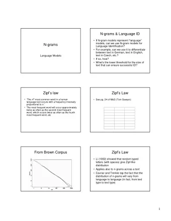
Zipf’s Law ¤ Zipf’s Law characterizes the relation between frequent and rare words: f(w) = C / r(w) or equivalently: f(w) * r(w) = C ¤ Frequency of lexical items (words types) in a large corpus is inversely proportional to their rank. ¤ Empirical observation in many different corpora ¤ Brown corpus: ¤ half of all types are hapax legomena 31

Effects of Zipf’s Law ¤ Lexicography: ¤ Sinclair (2005): need at least 20 instances ¤ BNC (10 8 Tokens): <14% of words appear 20 times or more ¤ Speech synthesis: ¤ may accept bad output for rare words ¤ but most words are rare! (at least 1 per sentence) ¤ Vocabulary growth: ¤ vocabulary growth of corpora is not constant ¤ G = #hapaxes / #tokens 32

Back to Language Models 33

Independence assumptions ¤ Let’s pretend that word at position t depends only on the words at positions t-1, t-2, ..., t-k for some fixed k ( Markov assumption of degree k). ¤ Then we get an n-gram model, with n = k+1: P(X t | X 1 ,...,X t-1 ) = P(X t | X t-k ,...,X t-1 ) for all t. ¤ Special names for unigram models (n = 1), bigram models (n = 2), trigram models (n = 3). 34

Independence assumption ¤ We assume independence of X t from events that are too far in the past, although we know that this assumption is incorrect. ¤ Typical tradeoff in statistical NLP: ¤ if model is too shallow, it won’t represent important linguistic dependencies ¤ if model is too complex, its parameters can’t be estimated accurately from the available data low n high n modeling errors estimation errors 35

Tradeoff in practice (Manning/Schütze, ch. 6) 36

Tradeoff in practice (Manning/Schütze, ch. 6) 37

Tradeoff in practice (Manning/Schütze, ch. 6) 38

Conclusion ¤ Statistical models of natural language ¤ Language models using n-grams ¤ Data sparseness is a problem. 39

next Tuesday ¤ smoothing language models 40