On Trades, Volume, and the Martingale Estimating Function Approach - PowerPoint PPT Presentation
On Trades, Volume, and the Martingale Estimating Function Approach for Stochastic Volatility Models with Jumps Friedrich Hubalek (Joint work with Petra Posedel) Johann Radon Institute for Computational and Applied Mathematics (RICAM) Special
On Trades, Volume, and the Martingale Estimating Function Approach for Stochastic Volatility Models with Jumps Friedrich Hubalek (Joint work with Petra Posedel) Johann Radon Institute for Computational and Applied Mathematics (RICAM) Special Semester on Stochastics with Emphasis on Finance Concluding Workshop Linz, December 2–4, 2008.
Our papers ◮ Friedrich Hubalek and Petra Posedel, Joint analysis and estimation of stock prices and trading volume in Barndorff-Nielsen and Shephard stochastic volatility models, arXiv:0807.3464 (July 2008) ◮ Friedrich Hubalek and Petra Posedel, Asymptotic analysis for a simple explicit estimator in Barndorff-Nielsen and Shephard stochastic volatility models, arXiv:0807.3479 (July 2008) ◮ Friedrich Hubalek and Petra Posedel, Asymptotic analysis for an optimal estimating function for Barndorff-Nielsen-Shephard stochastic volatility models, Work in progress.
The Barndorff-Nielsen and Shephard stochastic volatility models with jumps ◮ Logarithmic returns (discounted) � dX ( t ) = ( µ + β V ( t − )) dt + V ( t − ) dW ( t ) + ρ dZ λ ( t ) ◮ Instantaneous variance dV ( t ) = − λ V ( t − ) dt + dZ λ ( t ) W . . . Brownian motion, Z . . . subordinator, Z λ ( t ) = Z ( λ t ) [. . . ] ◮ Parameters: µ ∈ R . . . linear drift, β ∈ R . . . Itˆ o drift, ρ ∈ R . . . leverage, λ > 0. . . acf parameter.
Analytical tractability ◮ ( X ( t ) , V ( t ) , t ≥ 0). . . Markov, affine model (in continuous time) ◮ simple Riccati-type equations for characteristic resp. moment generating function ◮ general solution (up to one integral) ◮ Γ-OU and IG-OU completely explicitly in terms of elementary functions Exploited in ◮ Option pricing (Nicolato and Venardos) ◮ Portfolio optimization (Benth et al.) ◮ Minimum entropy martingale measure (Benth et al., Rheinl¨ ander and Steiger) ◮ Semimartingal Esscher transform (Hubalek and Sgarra) ◮ . . .
But statistical inference seems difficult! Bayesian, MCMC — computer intensive approaches! ◮ Barndorff-Nielsen O.E., Shephard N. (2001), Non-Gaussian Ornstein-Uhlenbeck-based models and some of their uses in financial economics. ◮ Roberts G.O., Papaspiliopoulos O., Dellaportas P. (2004), Bayesian inference for non-Gaussian Ornstein-Uhlenbeck stochastic volatility processes, ◮ J.E. Griffin, M.F.J. Steel (2006), Inference with non-Gaussian Ornstein-Uhlenbeck processes for stochastic volatility ◮ Matthew P.S. Gandera and David A. Stephens (2007), Stochastic volatility modelling in continuous time with general marginal distributions: Inference, prediction and model selection ◮ Sylvia Fr¨ uhwirth-Schnatter and Leopold S¨ ogner (2007?), Bayesian estimation of stochastic volatility models based on OU processes with marginal Gamma laws.
Discrete observations Grid t i = i δ , i ≥ 0, fixed width ∆ > 0, discrete time observations X i = X ( t i ) − X ( t i − 1 ) , V i = V ( t i ) Discrete dynamics � V i = e λ ∆ V i − 1 + U i X i = µ ∆ + β Y i + Y i W i + ρ Z i , Auxiliary quantities (no discretization error!) � t i e − λ ( t i − s ) dZ λ ( s ) Z i = Z λ ( t i ) − Z λ ( t i − 1 ) , U i = t i − 1 and � t i � t i 1 � √ Y i Y i = V ( s − ) ds , W i = V ( s − ) dW ( s ) . t i − 1 t i − 1 ( X i , V i , i ∈ N ). . . Markov affine model (in discrete time)
Construction and moments Two starting points ◮ L . . . infinitely divisible distribution on R + ⇒ subordinator Z with Z (1) d = L ⇒ (OU-L) ◮ D . . . self-decomposable distribution on R + ⇒ stationary Ornstein-Uhlenbeck process V with V ( t ) d = D ⇒ (D-OU) Moments of D resp. L → all (mixed, conditional, unconditional) integer moments by simple algebra (multivariate Faa di Bruno formula resp. Bell polynomials, practical calculations best by recursions!) E [ X n i ] , E [ V n i ] , E [ X m i V n i ] , E [ X ℓ i V m i V n i − 1 ] , E [ X n i | V i − 1 ] , E [ V n i | V i − 1 ] , E [ X m i V n i | V i − 1 ] , . . . ⇒ method of moments estimation
Various methods of moments ◮ Method of moments — MM (Pearson 1893) ◮ Generalized method of moments — GMM (Hansen 1982) ◮ Simulated method of moments — SMM (. . . ) ◮ Efficient method of moments — EMM (Gallant and Tauchen 1996), ◮ . . . ◮ [Methods of moments for weak convergence]
Estimation: Setting and problems Grid, fixed width, horizon (number of observations) going to Infinity for asymptotics! (Several other possibilities. . . ) ◮ Rich, well-informed financial institutions and traders observe and trade in continous-time ◮ Poor, academic statisticians and econometers do inference with daily (or less frequent!) observations ◮ [But: High-frequence analyses . . . ] Discrete time observations ⇒ V i not observed, BNS becomes non-Markovian, (a hidden Markov model)!
Remedies ◮ Substitute unobserved V i �→ model-implied ˆ V i from option data, i.e., joint analysis of P and Q . Cf. ◮ Jun Pan, The Jump-Risk Premia Implicit in Options: Evidence from an Integrated Time-Series Study (2002). (GMM, realistic, complicated, many assumptions.) Also our long term goal! ◮ Ignore the problem. Purely theoretical study, exhibits methodology, provides an upper bound for the accuracy for this type of methods. See our first paper! ◮ NOW: Substitute unobserved V i by an observable proxy, volume or number of trades.
Prices, volatility, trading intensity Our incentive ◮ Carl Lindberg, The estimation of the Barndorff-Nielsen and Shephard model from daily data based on measures of trading intensity. Applied Stochastic Models in Business and Industry 24 (4), 2008. Some earlier/classical references ◮ J. M. Karpoff, The relation between price changes and trading volume: a survey. JFQA 22, 1987. ◮ R.P.E. Gallant, A.R. and G. Tauchen, Stock prices and volume, Rev.Fin.Stud. 5:199–242, 1992. ◮ K.G. Jones, C. and M.L. Lipson, Transactions, volume and volatility. Rev.Fin.Stud. 7:631–651, 1994. ◮ G.E. Tauchen and M.Pitts, The Price Variability-Volume Relationship on Speculative Markets Econometrica 51,(1983).
The new variant/interpretation of the BNS models Bold simplification/assumption: Instantaneous variance IS a (constant) multiple of the trading volume resp. number of trades. Introduce a proportionality parameter σ > 0. [. . . ] ◮ Logarithmic returns � dX ( t ) = ( µ + β V ( t − )) dt + σ V ( t − ) dW ( t ) + ρ dZ λ ( t ) ◮ Trading volume (or number of trades) dV ( t ) = − λ V ( t − ) dt + dZ λ ( t ) W . . . Brownian motion, Z . . . subordinator, Z λ ( t ) = Z ( λ t ) [. . . ] ◮ Parameters: µ ∈ R . . . linear drift, β ∈ R . . . Itˆ o drift, σ > 0. . . proportionality, ρ ∈ R . . . leverage, λ > 0. . . acf parameter.
What about maximum likelihood ? ◮ Practical issue: Bivariate Markov, known transition probability (in terms of characteristic resp. cumulant function) ⇒ invert for each observation in each iterations [Possible remedies, approximate inversions, LeCam’s trick,. . . ] ◮ Theoretical issue: For infinite activity BDLP (e.g., IG-OU) fine, for finite activity (e.g., Γ-OU with exponential compound Poisson BDLP) P λ [ V 1 = ve − λ ∆ | V 0 = v ] = e − λ ∆ (no jump) ⇒ No dominating sigma-finite measure! ⇒ Usual ML framework does not apply! ◮ Generalized ML (Kiefer and Wolfowitz 1956) [. . . ] ◮ Much better than √ n by ad hoc (?) methods! [. . . ]
Martingale estimating functions E.g., Γ( ν, α )-OU: Parameter vector (3 + 4 = 7) θ = ( λ, ν, α, µ, β, σ, ρ ) Moments Ξ i = ( V i , V i V i − 1 , V 2 i , X i , X i V i − 1 , X i V i , X 2 Υ i = ( V i − 1 , V 2 i ) , i − 1 ) Martingale estimating function n G n ( θ ) = 1 � [Ξ i − f ( V i − 1 , θ )] , f ( v , θ ) = E θ [Ξ 1 | V 0 = v ] n i =1 Estimator: Solve G n ( θ ) = 0 ! Sample moments n n ξ n = 1 υ n = 1 � � Ξ i , Υ i , n n i =1 i =1
The explicit estimator n ) 2 > 0 ξ 2 n − ξ 1 n υ 1 n > 0 , υ 2 n − ( υ 1 � � Unique solution exists on C n = and is given by ζ n = γ n υ 1 n − ξ 1 n γ n = ( ξ 2 n − ξ 1 n υ 1 n ) / ( υ 2 n − ( υ 1 n ) 2 ); λ n = − log( γ n ) / ∆; − 1 + γ n n ) 2 − γ 2 η n = − ( − 1 + γ 2 n )( υ 1 n υ 2 n + ξ 3 n ǫ n = (1 − γ n ) /λ n ; − 1 + γ 2 n ( ξ 5 n − υ 1 n ξ 4 n ) β n = n ) 2 ); ǫ n ( υ 2 n − ( υ 1 n ) 2 + ǫ n λ n ( η n + ( υ 1 n ) 2 − υ 2 − β n ǫ n ( − ( υ 1 n ) + υ 2 n ) − ξ 1 n ξ 4 n + ξ 6 � � ρ n = / (2 ǫ n η n λ n ); n � − ∆ λ n ρ n ζ n − β n (∆ ζ n + ǫ n ( − ζ n + υ 1 n )) + ξ 4 � µ n = / ∆; n � b n = ∆ ζ n + ǫ n ( − ζ n + υ 1 σ n = a n / b n ; n ); a n = λ − 1 � 4 β n ( − ∆ + ǫ n ) η n λ n ρ n + β 2 n ( − 2∆ η n + ǫ n ( η n (2 + ǫ n λ n ) n n ) 2 − υ 2 n ) 2 + ξ 7 + ǫ n λ n (( υ 1 n ))) + λ n ( − 2∆ η n λ n ρ 2 n − ( ξ 4 � n ) ; Structure: First λ n , ν n , α n are simple AR(1) estimators, then µ n , β n , ρ n from a simple linear system, finally σ n from a quadratic equation.
Consistency The basic (and only!) assumption: V 0 self-decomposable rv on R + with E [ V n 0 ] < ∞ ∀ n ∈ N . The basic convergence result n 1 a . s . � X p i V q → E [ X p 1 V q i V r 1 V r − 0 ] ∀ p , q , r ∈ N . i − 1 n i =1 Remark: Ergodicity vs. simple proof. Martingale differences ⇒ uncorreclated ⇒ elementary convergence result. Theorem We have P ( C n ) → 1 and the estimator ˆ θ n is consistent on C n , namely a . s . ˆ θ n I C n − → θ 0 as n → ∞ .
Recommend
More recommend
Explore More Topics
Stay informed with curated content and fresh updates.
