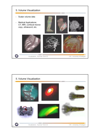
Volume Visualization Overview: Volume Visualization (1) - PowerPoint PPT Presentation

Volume Visualization

Overview: Volume Visualization (1) Introduction to volume visualization On volume data Voxels vs. cells Interpolation Gradient Classification Transfer Functions (TF) Slice vs surface vs. volume rendering Overview: techniques 2 Eduard Gröller, Helwig Hauser, Stefan Bruckner

Overview: Volume Visualization (2) Simple methods Slicing, multi-planar reconstruction (MPR) Direct volume visualization Image-order vs. object-order Raycasting a -compositing Hardware volume visualization Indirect volume visualization Marching cubes 3 Eduard Gröller, Helwig Hauser, Stefan Bruckner

Volume Visualization Introduction: VolVis = visualization of volume data Mapping 3D  2D Projection (e.g., MIP), slicing, vol. rendering, … Volume data = 3D  1D data Scalar data, 3D data space, space filling User goals: Gain insight in 3D data Structures of special interest + context 4 Eduard Gröller, Helwig Hauser, Stefan Bruckner

Volume Data Where do the data come from? Medical Application Computed Tomographie (CT) Magnetic Resonance Imaging (MR) Materials testing Industrial-CT Simulation Finite element methods (FEM) Computational fluid dynamics (CFD) etc. 5 Eduard Gröller, Helwig Hauser, Stefan Bruckner

3D Data Space How are volume data organized? Cartesian resp. regular grid: CT/MR: often dx=dy<dz, e.g. 135 slices (z) á 512² values (as x & y pixels in a slice) Data enhancement : iso-stack-calculation = Interpolation of additional slices, so that dx=dy=dz  512³ Voxel Data: Cells (cuboid), Corner: Voxel Curvi-linear grid resp. unstructured: Data organized as tetrahedra or hexahedra Often: conversion to tetrahedra 6 Eduard Gröller, Helwig Hauser, Stefan Bruckner

VolVis – Challenges Rendering projection, so much information and so few pixels! Large data sizes, e.g. 512  512  1024 voxel á 16 bit = 512 Mbytes Speed, Interaction is very important, >10 fps! 7 Eduard Gröller, Helwig Hauser, Stefan Bruckner

Voxels vs. Cells Two ways to interpret the data: Data: set of voxel Voxel = abbreviation for volume element (cf. pixel = "picture elem.) Voxel = point sample in 3D Not necessarily interpolated Data: set of cells Cell = cube primitive (3D) Corners: 8 voxel (see above) Values in cell: interpolation used 8 Eduard Gröller, Helwig Hauser, Stefan Bruckner

Interpolation 9 Eduard Gröller, Helwig Hauser, Stefan Bruckner

Interpolation – Results 10 Eduard Gröller, Helwig Hauser, Stefan Bruckner

Higher-Order Reconstruction (1) If very high quality is needed, more complex reconstruction filters may be required Marschner-Lobb function is a common test signal to evaluate the quality of reconstruction filters [Marschner and Lobb 1994] The signal has a high amount of its energy near its Nyquist frequency Makes it a very demanding test for accurate reconstruction 11 Eduard Gröller, Helwig Hauser, Stefan Bruckner

Higher-Order Reconstruction (2) Analytical evaluation of the Marschner-Lobb test signal 12 Eduard Gröller, Helwig Hauser, Stefan Bruckner

Higher-Order Reconstruction (3) Trilinear reconstruction of Marschner-Lobb test signal 13 Eduard Gröller, Helwig Hauser, Stefan Bruckner

Higher-Order Reconstruction (4) B-Spline reconstruction of Marschner-Lobb test signal 14 Eduard Gröller, Helwig Hauser, Stefan Bruckner

Higher-Order Reconstruction (5) Windowed sinc reconstruction of Marschner- Lobb test signal 15 Eduard Gröller, Helwig Hauser, Stefan Bruckner

Gradients in Volume Data Volume data: f( x )  R 1 , x  R 3 Gradient  f: 3D vector points in direction of largest function change Gradient magnitude: length of gradient Emphasis of changes: Special interest often in transitional areas Gradients: measure degree of change (like surface normal) Larger gradient magnitude  larger opacity 16 Eduard Gröller, Helwig Hauser, Stefan Bruckner

Gradients as Normal Vector Replacement Gradient  f = (  f/  x,  f/  y,  f/  z)  f| x0 normal vector to iso-surface f(x 0 )=f 0 Central difference in x-, y- & z-direction (in voxel):  f(x  1)  f(x  1)   f (x,y,z) = 1/2  f(y  1)  f(y  1)   f(z  1)  f(z  1)  Then tri-linear interpolation within a cell Alternatives:  f (x)=f(x  1)  f(x) Forward differencing: Backwards differencing:  f (x)=f(x)  f(x  1)  f (x  0.5)=f(x  1)  f(x) Intermediate differencing: 17 Eduard Gröller, Helwig Hauser, Stefan Bruckner

Classification Assignment data  semantics: Assignment to objects, e.g., bone, skin, muscle, etc. Usage of data values, gradient, curvature Goal: segmentation Often: semi-automatic resp. manual Automatic approximation: transfer functions (TF) 18 Eduard Gröller, Helwig Hauser, Stefan Bruckner

Transfer Functions (TF) Mapping data  ”renderable quantities”: 1.) data  color (f(i)  C(i)) 2.) data  opacity (non-transparency) (f(i) a (i)) opacity “bone” red, opaque “skin” yellow, semi-transparent “air” data values color 19 Eduard Gröller, Helwig Hauser, Stefan Bruckner

Different Transfer Functions Image results: Strong dependence on transfer functions Non-trivial specification Limited segmentation possibilities 20 Eduard Gröller, Helwig Hauser, Stefan Bruckner

Lobster – Different Transfer Functions Three objects: media, shell, flesh 21 Eduard Gröller, Helwig Hauser, Stefan Bruckner

Concepts and Terms sampled data analytical data (measurement) (modelling) iso-surfacing voxel space geometric surfaces (discrete) (analytic) voxelization (direct) volume surface rendering rendering pixel space (discrete) 22 Eduard Gröller, Helwig Hauser, Stefan Bruckner

Concepts and Terms Example sampled data analytical data (measurement) (modelling) X-Ray iso-surfacing voxel space geom. surfaces Modelling (discrete) (analytic) voxelization volume surface Surface- rendering rendering pixel space (discrete) definition Sampling (voxelization), combination Direct volume rendering 23 Eduard Gröller, Helwig Hauser, Stefan Bruckner

Slice vs. Surface vs. Volume Rendering Slice rendering 2D cross-section from 3D volume data Surface rendering: Indirect volume visualization Intermediate representation: iso- surface, “3D” Pros: Shading  Shape!, HW-rendering Volume rendering: Direct volume visualization Usage of transfer functions Pros: illustrate the interior, semi-transparency 24 Eduard Gröller, Helwig Hauser, Stefan Bruckner

Slices vs. Iso-Surfaces. vs. Volume Rendering Comparison ozon-data over Antarctica: Slices: selective (z), 2D, color coding Iso-surface: selective (f 0 ), covers 3D Vol. rendering: transfer function dependent, “(too) sparse – (too) dense” 25 Eduard Gröller, Helwig Hauser, Stefan Bruckner

VolVis-Techniques – Overview Simple methods: Slicing, MPR (multi-planar reconstruction) Direct volume visualization: Ray casting Shear-warp factorization Splatting 3D texture mapping Fourier volume rendering Surface-fitting methods: Marching cubes (marching tetrahedra) 26 Eduard Gröller, Helwig Hauser, Stefan Bruckner

Simple Methods Slicing, etc.

Slicing Slicing: Axes-parallel slices Regular grids: simple Without transfer function no color Windowing: adjust contrast General grid, arbitrary slicing direction Window white black data values 28 Eduard Gröller, Helwig Hauser, Stefan Bruckner

Direct Volume Visualization

Image-Order vs. Object-Order 30 Eduard Gröller, Helwig Hauser, Stefan Bruckner

Image-Order vs. Object-Order 31 Eduard Gröller, Helwig Hauser, Stefan Bruckner

Ray Casting Image-Order Method

Ray Tracing vs. Ray Casting Ray Tracing: method from image generation In volume rendering: only viewing rays  therefore Ray Casting Classical image-order method Ray Tracing: ray – object intersection Ray Casting: no objects, density values in 3D In theory: take all data values into account! In practice: traverse volume step by step Interpolation necessary for each step! 33 Eduard Gröller, Helwig Hauser, Stefan Bruckner

Ray Traversal through Volume Data Context: Volume data: 1D value defined in 3D – f( x )  R 1 , x  R 3 Ray defined as half-line: r (t)  R 3 , t  R 1 >0 Values along Ray: f( r (t))  R 1 , t  R 1 >0 (intensity profile) 34 Eduard Gröller, Helwig Hauser, Stefan Bruckner

Standard Ray Casting Lev oy ’88: 1. C(i), a (i) (from TF) 2. Ray casting, interpolation 3. Compositing (or combinations) 35 Eduard Gröller, Helwig Hauser, Stefan Bruckner

1. Shading, Classification 1. Step: Shading, f(i)  C(i): Apply transfer function diffuse illumination (Phong), gradient  normal Classification, f(i) a (i): Levoy ’88, gradient enhanced Emphasizes transitions Nowadays: shading/classification after ray-casting/resampling 36 Eduard Gröller, Helwig Hauser, Stefan Bruckner

2. Ray Traversal Cast ray through the volume and perform sampling at discrete positions image plane eye data set 37 Eduard Gröller, Helwig Hauser, Stefan Bruckner

2. Ray Traversal – Three Approaches equidistant samples all voxels used once samples weighted by lengths of ray segments 38 Eduard Gröller, Helwig Hauser, Stefan Bruckner