Multi-layer Perceptrons & the Back-propagation Algorithm - PDF document

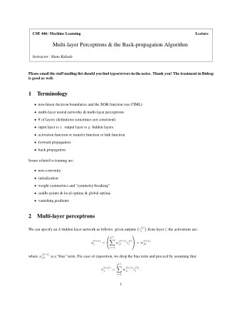
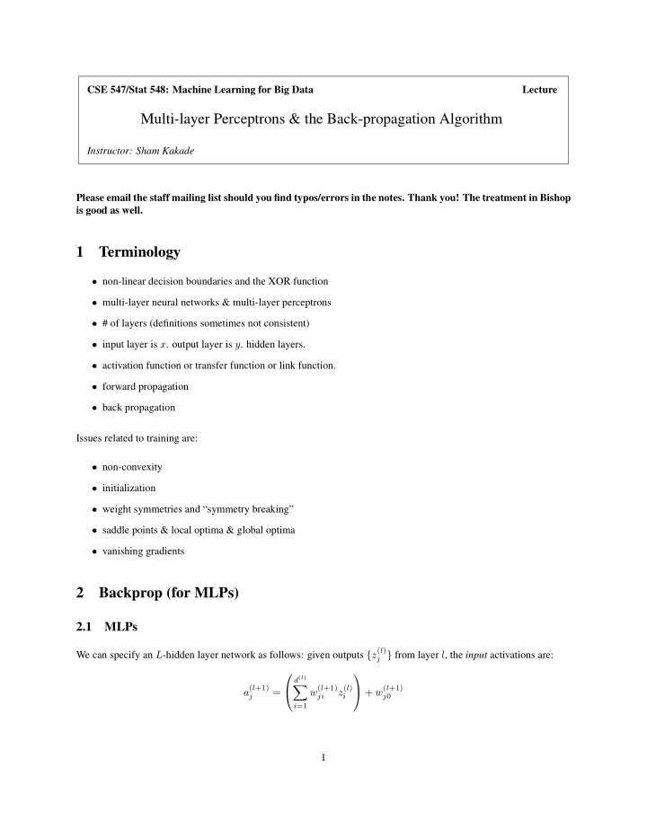
CSE 547/Stat 548: Machine Learning for Big Data Lecture Multi-layer Perceptrons & the Back-propagation Algorithm Instructor: Sham Kakade Please email the staff mailing list should you find typos/errors in the notes. Thank you! The treatment in Bishop is good as well. 1 Terminology • non-linear decision boundaries and the XOR function • multi-layer neural networks & multi-layer perceptrons • # of layers (definitions sometimes not consistent) • input layer is x . output layer is y . hidden layers. • activation function or transfer function or link function. • forward propagation • back propagation Issues related to training are: • non-convexity • initialization • weight symmetries and “symmetry breaking” • saddle points & local optima & global optima • vanishing gradients 2 Backprop (for MLPs) 2.1 MLPs We can specify an L -hidden layer network as follows: given outputs { z ( l ) j } from layer l , the input activations are:   d ( l ) � a ( l +1) w ( l +1) z ( l )  + w ( l +1)  = j 0 j ji i i =1 1

where w ( l +1) is a “bias” term. For ease of exposition, we drop the bias term and proceed by assuming that: j 0 d ( l ) � a ( l +1) w ( l +1) z ( l ) = . j ji i i =1 The output activation of each node is: z ( l +1) = h ( a ( l +1) ) j j Remark: The terminology of the “activation” is not necessarily used consistently. Sometimes the activation is used to refer to only the input a ’s , as defined above, or only the input z ’s, as defined above . Sometimes the literature uses the terminology input activation and output activation. We will use the latter terminology as it less confusing. Or we just use the terminology “inputs” and “outputs” of nodes. The target function, after we go through L -hidden layers, is then: d ( L ) � y ( x ) = a ( L +1) = w ( L +1) z ( L ) � , i i i =1 where saying the output is the activation at level L + 1 . It is straightforward to generalize this to force � y ( x ) to be bounded between 0 and 1 (using a sigmoid transfer function) or having multiple outputs. Let us also use the convention that: z (0) = x [ i ] i The parameters of the model are all the weights w ( L +1) , w ( L ) , . . . w (1) . 2.2 The Back-Propagation Algorithm for MLPs In general, the loss function in an L -hidden layer network is: � L ( w (1) , w (2) , . . . , w ( L +1) ) = 1 ℓ ( y, � y ( x )) N n and for the special case of the square loss we have: � � 1 y ( x n )) = 1 1 y ( x n )) 2 ℓ ( y n , � ( y n − � N 2 N n n Again, we seek to compute: ∇ ℓ ( y n , � y ( x n )) where the gradient is with respect to all the parameters. The Forward Pass Starting with the input x , go forward (from the input to the output layer), compute and store in memory the variables a (1) , z (1) , a (2) , z (2) , . . . a ( L ) , z ( L ) , a ( L +1) 2

The Backward Pass Note ℓ ( y, � y ) depends on all the parameters and we will not write out this functional dependency (e.g. � y depends on x and all the weights). We will compute the derivates by recursion. It useful to do recursion by computing the derivates with respect to the input activations and proceeding “backwards” (from the output layer to the input layer). Define: := ∂ℓ ( y, � y ) δ ( l ) j ∂a ( l ) j First, let us see that if we had all the δ ( l ) j ’s then we are able to obtain the derivatives with respect to all of our parameters: ∂a ( l ) ∂ℓ ( y, � y ) = ∂ℓ ( y, � y ) j = δ ( l ) j z ( l − 1) i ∂w ( l ) ∂a ( l ) ∂w ( l ) ji j ji ∂∂a ( l ) = z ( l − 1) where we have used the chain rule and that j . To see the latter claim is true, note ∂w ( l ) i ji d ( l − 1) � a ( l ) w ( l ) jc z ( l − 1) = c j c =1 ∂∂a ( l ) = z ( l − 1) (the sum is over all nodes c in layer l − 1 ). This expression implies j ∂w ( l ) i ji Now let us understand how to start the recursion, i.e. to compute the δ ’s for the output layer, as there is only one node y = a ( L +1) , and � δ ( L +1) = ∂ℓ ( y, � y ) ∂a ( L +1) = − ( y − � y ) (so we don’t need a subscript of j since there is only one node). Hence, for the output layer, ∂ℓ ( y, � y ) = δ ( L +1) z ( L ) y ) z ( L ) = − ( y − � j j ∂w ( L +1) j where we have used our expression for δ ( L +1) . Thus, we know how to start our recursion. Now let us proceed recursively, computing δ ( l ) using δ ( l +1) . Observe that j j all the functional dependencies on the activations at layer l goes through the activations at l + 1 . This implies, using the chain rule, ∂ℓ ( y, � y ) δ ( l ) = j ∂a ( l ) j d ( l +1) ∂a ( l +1) � ∂ℓ ( y, � y ) k = ∂a ( l +1) ∂a ( l ) k =1 k j d ( l +1) � ∂a ( l +1) δ ( l +1) k = k ∂a ( l ) k =1 j To complete the recursion we need to evaluate ∂a ( l +1) . By definition, k ∂a ( l ) j d ( l ) d ( l ) � � a ( l +1) w ( l +1) w ( l +1) z ( l ) h ( a ( l ) = = c ) c k kc kc c =1 c =1 3

This implies: ∂a ( l +1) = w ( l +1) h ′ ( a ( l ) k j ) , kj ∂a ( l ) j and, by substitution, d ( l +1) � δ ( l ) = h ′ ( a ( l ) w ( l +1) δ ( l +1) j ) j kj k k =1 which completes our recursion. 2.3 The Algorithm We are now ready to state the algorithm. The Forward Pass: 1. Starting with the input x , go forward (from the input to the output layer), compute and store in memory the variables a (1) , z (1) , a (2) , z (2) , . . . a ( L ) , z ( L ) , a ( L +1) The Backward Pass: 1. Initialize as follows: δ ( L +1) = − ( y − � y ) = − ( y − a ( L +1) ) and compute the derivatives at the output layer: ∂ℓ ( y, � y ) y ) z ( L ) = − ( y − � j ∂w ( L +1) j 2. Recursively, compute d ( l +1) � δ ( l ) = h ′ ( a ( l ) w ( l +1) δ ( l +1) j ) j kj k k =1 and also compute our derivatives at layer l : ∂ℓ ( y, � y ) = δ ( l ) j z ( l − 1) i ∂w ( l ) ji 3 Time Complexity Assume that addition, subtraction, multiplication, and division take “one unit” of time (and let us ignore numerical precision issues). Let us say the time complexity to compute ℓ ( y, � y ( x )) is based on the naive algorithm (which explicitly just computes all the sums in the forward pass). Theorem 3.1. Suppose that we can compute the derivative h ′ ( · ) in an amount of time that is within a constant factor of the time it takes to compute h ( · ) itself (and suppose that constant is 5 ). Using the backprop algorithm, the (total) time to compute both ℓ ( y, � y ( x )) and ∇ ℓ ( y, � y ( x )) — note that ∇ ℓ ( y, � y ( x )) contains # parameter partial derivatives — is within a factor of 5 of computing just the scalar value ℓ ( y, � y ( x )) . 4

Proof. The number of transfer function evaluations in the forward pass is just the number of nodes. In the backward pass, the number of times we need to evaluate the derivative of the transfer function is also just the number of nodes. In the forward pass, note that the total computation time is a constant factor (actually 2 ) times the number weights. To see this, note that to compute any activation, it costs us (one addition and one multiplication) associated with each weight (and that the every weight is only involved in the computation of just one activation). Similarly, by examining the recursion in the backward pass, we see that the total compute time to get all the δ ’s is a constant factor times the number of weights (again there is only one multiplication and one addition associated with each weight). Also, the compute time for obtaining the partial derivatives from the δ ’s is equal to the number of weights. Remark: That we defined the time complexity to be under the “naive” algorithm is irrelevant. If we had a faster algorithm to compute ℓ ( y, � y ( x )) (say through a faster matrix multiplication algorithm or possibly other tricks), then the above theorem would still hold. This is the remarkable Baur-Strassen theorem [1] (also independently stated by [2]). References [1] Walter Baur and Volker Strassen. The complexity of partial derivatives. Theoretical Computer Science , 22:317– 330, 1983. [2] Andreas Griewank and Andrea Walther. Evaluating Derivatives: Principles and Techniques of Algorithmic Dif- ferentiation . Society for Industrial and Applied Mathematics, Philadelphia, PA, USA, second edition, 2008. 5