Multi-layer Perceptrons & the Back-propagation Algorithm - PDF document

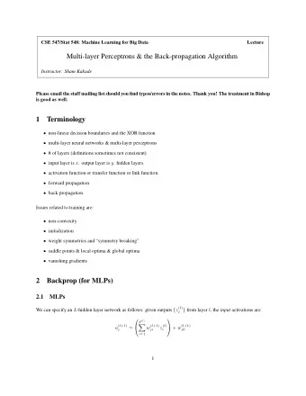
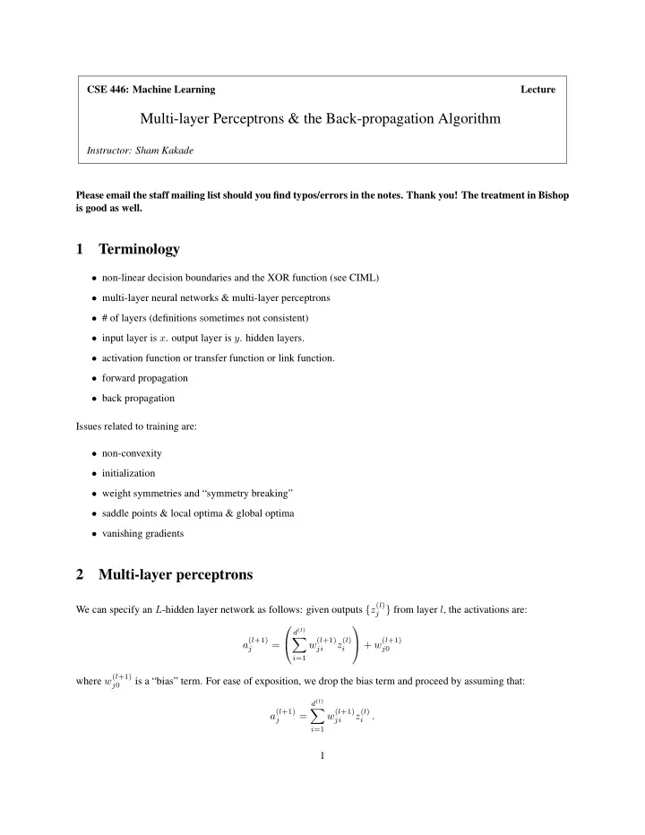
CSE 446: Machine Learning Lecture Multi-layer Perceptrons & the Back-propagation Algorithm Instructor: Sham Kakade Please email the staff mailing list should you find typos/errors in the notes. Thank you! The treatment in Bishop is good as well. 1 Terminology • non-linear decision boundaries and the XOR function (see CIML) • multi-layer neural networks & multi-layer perceptrons • # of layers (definitions sometimes not consistent) • input layer is x . output layer is y . hidden layers. • activation function or transfer function or link function. • forward propagation • back propagation Issues related to training are: • non-convexity • initialization • weight symmetries and “symmetry breaking” • saddle points & local optima & global optima • vanishing gradients 2 Multi-layer perceptrons We can specify an L -hidden layer network as follows: given outputs { z ( l ) j } from layer l , the activations are:   d ( l ) � a ( l +1) w ( l +1) z ( l )  + w ( l +1)  = j ji i j 0 i =1 where w ( l +1) is a “bias” term. For ease of exposition, we drop the bias term and proceed by assuming that: j 0 d ( l ) � a ( l +1) w ( l +1) z ( l ) = . j ji i i =1 1

The output of each node is: z ( l +1) = h ( a ( l +1) ) j j The target function, after we go through L -hidden layers, is then: d ( L ) � y ( x ) = a ( L +1) = w ( L +1) z ( L ) � , i i i =1 where saying the output is the activation at level L + 1 . It is straightforward to generalize this to force � y ( x ) to be bounded between 0 and 1 (using a sigmoid transfer function) or having multiple outputs. Let us also use the convention that: z (0) = x [ i ] i The parameters of the model are all the weights w ( L +1) , w ( L ) , . . . w (1) . 3 The Back-Propagation Algorithm In general, the loss function in an L -hidden layer network is: � L ( w (1) , w (2) , . . . , w ( L +1) ) = 1 ℓ ( y, � y ( x )) N n and for the special case of the square loss we have: � � 1 y ( x n )) = 1 y ( x n )) 2 ℓ ( y n , � ( y n − � N N n n Again, we seek to compute: ∇ ℓ ( y n , � y ( x n )) where the gradient is with respect to all the parameters. The Forward Pass Starting with the input x , go forward (from the input to the output layer), compute and store in memory the variables a (1) , z (1) , a (2) , z (2) , . . . a ( L ) , z ( L ) , a ( L +1) The Backward Pass Note ℓ ( y, � y ) depends on all the parameters and we will not write out this functional dependency (e.g. � y depends on x and all the weights). We will compute the derivates by recursion. It useful to do recursion by computing the derivates with respect to the activations and proceeding “backwards” (from the output layer to the input layer). Define: := ∂ℓ ( y, � y ) δ ( l ) j ∂a ( l ) j 2

First, let us see that if we had all the δ ( l ) j ’s then we are able to obtain the derivatives with respect to all of our parameters: ∂a ( l ) ∂ℓ ( y, � y ) = ∂ℓ ( y, � y ) j = δ ( l ) j z ( l − 1) i ∂w ( l ) ∂a ( l ) ∂w ( l ) ji j ji ∂∂a ( l ) = z ( l − 1) j where we have used the chain rule and that . To see the latter claim is true, note ∂w ( l ) i ji d ( l − 1) � a ( l ) w ( l ) jc z ( l − 1) = j c c =1 ∂∂a ( l ) = z ( l − 1) (the sum is over all nodes c in layer l − 1 ). This expression implies j i ∂w ( l ) ji Now let us understand how to start the recursion, i.e. to compute the δ ’s for the output layer, as there is only one node y = a ( L +1) , and � δ ( L +1) = ∂ℓ ( y, � y ) = − ( y − � y ) ∂a ( l ) (so we don’t need a subscript of j since there is only one node). Hence, for the output layer, ∂ℓ ( y, � y ) = δ ( L +1) z ( L ) y ) z ( L ) = − ( y − � j j ∂w ( L +1) j where we have used our expression for δ ( L +1) . Thus, we know how to start our recursion. Now let us proceed recursively, computing δ ( l ) using δ ( l +1) . Observe that j j all the functional dependencies on the activations at layer l goes through the activations at l + 1 . This implies, using the chain rule, ∂ℓ ( y, � y ) δ ( l ) = j ∂a ( l ) j d ( l +1) � ∂a ( l +1) ∂ℓ ( y, � y ) k = ∂a ( l +1) ∂a ( l ) k =1 j k d ( l +1) � ∂a ( l +1) δ ( l +1) k = k ∂a ( l ) k =1 j To complete the recursion we need to evaluate ∂a ( l +1) k . By definition, ∂a ( l ) j d ( l ) d ( l ) � � a ( l +1) w ( l +1) w ( l +1) z ( l ) h ( a ( l ) = = c ) c k kc kc c =1 c =1 This implies: ∂a ( l +1) = w ( l +1) h ′ ( a ( l ) k j ) , kj ∂a ( l ) j and, by substitution, d ( l +1) � δ ( l ) = h ′ ( a ( l ) w ( l +1) δ ( l +1) j ) j kj k k =1 which completes our recursion. 3

3.1 The Algorithm We are now ready to state the algorithm. The Forward Pass: 1. Starting with the input x , go forward (from the input to the output layer), compute and store in memory the variables a (1) , z (1) , a (2) , z (2) , . . . a ( L ) , z ( L ) , a ( L +1) The Backward Pass: 1. Initialize as follows: δ ( L +1) = − ( y − � y ) = − ( y − a ( L +1) ) and compute the derivatives at the output layer: ∂ℓ ( y, � y ) y ) z ( L ) = − ( y − � j ∂w ( L +1) j 2. Recursively, compute d ( l +1) � δ ( l ) = h ′ ( a ( l ) w ( l +1) δ ( l +1) j ) j kj k k =1 and also compute our derivatives at layer l : ∂ℓ ( y, � y ) = δ ( l ) j z ( l − 1) i ∂w ( l ) ji 4