Modelling of Packet Loss in an Asynchronous Packet Switch using - PowerPoint PPT Presentation
Modelling of Packet Loss in an Asynchronous Packet Switch using PEPA Wim Vanderbauwhede Department of Computing Science University of Glasgow September 6, 2005- WV 1 Overview Asynchronous Packet Switch Building the PEPA Model
Modelling of Packet Loss in an Asynchronous Packet Switch using PEPA Wim Vanderbauwhede Department of Computing Science University of Glasgow September 6, 2005- WV 1
Overview � Asynchronous Packet Switch � Building the PEPA Model � Some Results � Conclusion
Asynchronous Packet Switch (1)
Asynchronous Packet Switch (2) Basic Functionality � Switches data packets between ports � Contention occurs when two or more packets want to occupy the same destination port � Buffering is used to resolve contention
Asynchronous Packet Switch (3) Properties � Store-and-forward: packet is stored in buffer cell, then for- warded � Packet must have left buffer cell completely before another packet can occupy the same cell � Simultaneous egress from buffers is possible (transparent) � Switch fabric is a black box
Asynchronous Packet Switch (4) Schematic
Asynchronous Packet Switch (5) Steady-State Packet Loss � Important performance measure for packet switch � Depends on load and buffer depth, � But also on traffic distribution and switch architecture. � PEPA is useful to analyse the former, for the latter a DES is required.
Asynchronous Packet Switch (6) Queue Model for Packet Switch The switch can be modelled as a system of c interacting M / M / c / N queues:
The PEPA Model for the Switch Organisation of the PEPA Model G: traffic generator; Q: buffer queue; M: output multiplexer //: components in parallel (empty interaction) → : direction of active/passive interaction
Building the Model - Traffic generator Two-state traffic generator � Models packet traffic for packets with variable length and inter- arrival time � We use following definitions: τ on , τ of f : time period during which the source is on resp. o f f . λ on = 1 / τ on , λ of f = 1 / τ of f : the corresponding rates � Model: G = ( of f , λ of f ) . ( on , λ on ) . G
Building the Model - Buffer system (1) Buffer System Model: Definitions and Notations � Define the base state Q i as the set of states in which i out of N buffers are occupied � Let j be the number of packets entering the buffer, k the num- ber of packet leaving the buffer. � We introduce following notation: + j − k i , i ∈ { 0 ,..., N } ; j ∈ { 0 , 1 } ; k ∈ { 0 ,..., c } Q � Read as: "The queue Q has i filled buffers, j packets are arriv- ing and k are leaving"
Building the Model - Buffer system (2) Analysis of states and transitions for a single M/M/c/N queue � Example for M/M/1/N queue
Building the Model - Buffer system (3) Actions and Rates � State transitions are caused by the arrival of a packet or the arrival of a signal telling a packet to leave. � Presence/absence of a packet at the ingress/egress port is modelled by the actions { on , of f } { in , out } with corresponding rates λ { on , of f } , { in , out } � Buffer filling rate λ on , in : models the packet length, and therefore λ on , in ≡ λ on , out . � Signalling rate λ of f , out : models the delay between the the egress port becoming free and the packet starting to leave the buffer.
Building the Model - Buffer system (4) Model for single egress ( c = 1 ): + 0 + 1 + 0 − 0 − 0 − 1 = ( o f f in , λ of f , in ) . Q +( of f out , λ of f , out ) . Q Q i i i + 1 + 0 + 1 − 0 − 0 − 1 = ( on in , λ on , in ) . Q i + 1 +( of f out , λ of f , out ) . Q Q i i + 0 + 1 + 0 − 1 − 1 − 0 = ( of f in , λ of f , in ) . Q +( on out , λ on , out ) . Q Q i − 1 i i + 1 + 0 + 1 − 1 − 1 − 0 = ( on in , λ on , in ) . Q i + 1 +( on out , λ on , out ) . Q Q i − 1 i
Building the Model - Buffer system (5) Introducing Drop States � We are interested in the packet loss in steady state . � We calculate this as sum of the probabilities of being in a state where the packet is being dropped. � To do so, we must introduce “ drop states ”. � The full state ( i = N ) leads to a drop state on arrival of a packet: + 0 + 1 + 0 − 0 − 0 − 1 N = ( o f f in , λ of f , in ) . Q N , d +( of f out , λ of f , out ) . Q Q N + 0 + 1 + 0 − 1 − 1 − 0 N = ( of f in , λ of f , in ) . Q N , d +( on out , λ on , out ) . Q Q N − 1
Building the Model - Buffer system (5) � All base states ( 0 < i ≤ N ) gain 2 drop states: while the packet is being dropped, a packet can start/stop leaving the buffer, leading to a lower base state. + 1 + 0 + 1 − 0 − 0 − 1 i , d = ( on in , λ on , in ) . Q +( of f out , λ of f , out ) . Q Q i i , d + 1 + 0 + 1 − 1 − 1 − 0 i , d = ( on in , λ on , in ) . Q +( on out , λ on , out ) . Q Q i − 1 , d i
Building the Model - Buffer system (6) Multiple Egress Model: � Let m = min ( N , c ) and λ { on , of f } , out , k = k . λ { on , of f } , out . � The previous equations change to ( 0 < i < N , 0 < k < m ): + 0 + 1 + 0 − k − k − ( k − 1 ) = ( o f f in , λ of f , in ) . Q +( on out , λ on , out , k ) . Q Q i − 1 i i + 0 − ( k + 1 ) +( of f out , λ of f , out , m − k ) . Q i + 1 + 0 + 1 − k − k − ( k − 1 ) = ( o f f in , λ of f , in ) . Q i + 1 +( on out , λ on , out , k ) . Q Q i − 1 i + 1 − ( k + 1 ) +( of f out , λ of f , out , m − k ) . Q i
Building the Model - Buffer system (7) Multiple Egress Drop States � For 0 < i ≤ N , 0 < k < m + 1 + 0 + 1 − k − k − ( k − 1 ) i , d = ( o f f in , λ of f , in ) . Q +( on out , λ on , out , k ) . Q Q i − 1 , d i + 1 − ( k + 1 ) +( of f out , λ of f , out , m − k ) . Q i , d � For 0 < i ≤ N , k = 0 + 1 + 0 + 1 − 0 − 0 − 1 i , d = ( o f f in , λ of f , in ) . Q +( of f out , λ of f , out , m − k ) . Q Q i , d i � For 0 < i ≤ N , k = m + 1 + 0 + 1 − m − m − ( m − 1 ) i , d = ( o f f in , λ of f , in ) . Q +( on out , λ on , out , k ) . Q Q i − 1 , d i
Building the Model - Complete Switch Modelling Interacting Queues � To combine C of the above queues Q c with c outputs into a switch, we first introduce a multiplexer M: M = ( on out , ⊤ ) . ( of f out , λ of f , out ) . M � The final switch consists of C cooperations of G and Q c in par- allel, cooperating with c multiplexers in parallel S c = G onin , o f fin Q c ⊲ ⊳ Switch = ( S c � ... � S c ) onout , o f fout ( M � ... � M ) ⊲ ⊳
Using the PEPA Model Toolchain for this work � PEPA Workbench to calculate the TRM � MatLab to calculate the steady-state solution � A Perl script to drive the simulation: � generate the input file for the PEPA Workbench & run � generate a MatLab file & run � calculate the packet loss probability from the steady-state � The Simulation::Automate Perl package to automate the DOE
Some Results (1) 1 Influence of the Signalling Delay ( λ of f , out )
Some Results (2) Comparison with Discrete Event Simulator
Some Results (3) Comparison with Rate-based Model
Conclusion � A methodology for analytical modelling of steady-state packet loss in an asynchronous packet switch � For asynchronous buffered switches, the state space is very large � Building a PEPA model with explicit states is non-trivial
Appendix: Rate-based Model (1) Rate-Based PEPA Model � Define a traffic generator generating packets at rate λ : G = ( in , λ ) . G � And a multiplexer taking in packets at rate µ , defined as λ ρ , with ρ the load: M = ( out , µ ) . M
Appendix: Rate-based Model (2) � The queue model is: Q 0 = ( in , λ ) . Q 1 Q i = ( in , ⊤ ) . Q i + 1 +( out , µ ) . Q i − 1 , 0 < i < N Q N = ( in , ⊤ ) . Q Nd +( out , µ ) . Q N − 1 Q Nd = ( in , ⊤ ) . Q Nd +( out , µ ) . Q N − 1
Recommend
More recommend
Explore More Topics
Stay informed with curated content and fresh updates.

