Modeling, Analysis and Control Radu Grosu Vienna University of - PowerPoint PPT Presentation
Hybrid Systems Modeling, Analysis and Control Radu Grosu Vienna University of Technology Lecture 6 Continuous AND Discrete Systems Control Theory Computer Science Continuous systems Discrete systems approximation, stability abstraction,
Hybrid Systems Modeling, Analysis and Control Radu Grosu Vienna University of Technology Lecture 6
Continuous AND Discrete Systems Control Theory Computer Science Continuous systems Discrete systems approximation, stability abstraction, composition control, robustness concurrency, verification Hybrid Systems Software controlled systems Embedded real-time systems Multi-agent systems
Models and Tools Dynamic systems with continuous & discrete state variables Continuous Part Discrete Part Differential equations, Automata, Petri nets, Models transfer functions, Statecharts, Lyapunov functions, Boolean algebra, formal Analytical Tools eigenvalue analysis, logics, verification, Matlab, Matrix x , Statemate, Rational Software Tools VisSim, Rose, SMV,
Modeling a Hybrid System Model of System Model of Model of Physics Software continuous dynamics discrete dynamics
Hybrid Automaton (HA) locations or modes guard (discrete states) edge n x inv ( n ) e : guard ( x ) 0 m action ( x, x ) x inv ( m ) x init ( m ) jump transformation invariant: HA may remain in initial m as long as x inv ( m ) condition continuous dynamics
Example: Bouncing Ball Ball has mass m and position x Ball initially at position x 0 and at rest Ball bounces when hitting ground at x 0
Bouncing Ball: Free Fall Condition for free fall: x 0 Differential equations: First order
Bouncing Ball: Bouncing Condition for bouncing: x 0 Action for bouncing: v c v Coefficient c: deformation, friction
Bouncing Ball: Hybrid Automaton x x 0 , v 0 initial condition location freeFall x 0 invariant discrete transition flow label bounce: guard v c v action
Bouncing Ball: Associated Program initial condition location freeFall invariant discrete transition flow label bounce: guard v c v action
Execution of Bouncing Ball x (t) 0 Position ( x ) x (t) 1 x (t) 2 x (t) x (t) 3 4 T T T 3 T T Time ( t ) 0 1 2 4 Velocity ( v ) v (t) v (t) 4 v (t) 3 v (t) 2 v (t) 1 0 T T T T 3 T Time ( t ) 0 1 2 4
Boost DC-DC Converter i L i 0 v c v 0 s 0 s 0
Boost DC-DC Converter i L i 0 v c v 0 s 1 s 0 s 1 s 1 s 0 s 0
Boost DC-DC Converter i L i 0 v c v 0 s 1 s 0 s 1 s 0 s 1 s 0 float i L i 0 , v c v 0 , d d 0 ; bool s 0; while true { while ( s 0) { R L L i L 1 i L i L ( L v S ) d v C v C 1 1 C v C d R C R 0 read( s ) }
Execution of Boost DC-DC Converter Capacitor Voltage and Inductor Current 16 200 Parameters : Current i L , mA , V U s = 20 V 12 150 Voltage u C þ L = 1 mH 8 100 C = 50 nF 4 50 L = 1 k W 0 0 R 0 1 2 3 C = 10 W R Time t , ms 0 = 10 k W R Load Voltage dt = 200 ns 16 200 Current i L , mA Voltage u R 0 , V U max = 16 V 12 150 U min = 14 V 8 100 4 50 0 0 0 1 2 3 Time t , ms
Hybrid Automaton H Variables: Continuous variables x [ x 1 ,..., x n ] Control Graph: Finite directed multigraph ( V , E ) Finite set V of control modes Finite set E of control switches Vertex labeling functions: for each v V Initial states: init( v )( x ) defines initial region Invariant: inv( v )( x ) defines invariant region Edge labeling functions: for each e E Guard: guard( e )( x ) defines enabling region Update: action( e )( x, x ) defines the reset region Synchronization labels: label( e ) defines communication
Executions of a Hybrid Automaton State: ( m , x ) such that x inv( m ) Initialization: ( m , x ) such that x init( m ) Two types of state updates: Discrete switches: ( m , x ) a ( m , x ) if e ( m,m') E label( e ) a guard( e )( x ) 0 action(e)( x , x ) Continuous flows: ( m , x ) f ( m , x ) if f : [0,T] R n . f (0) x f (T) x
Recommend


More recommend
Explore More Topics
Stay informed with curated content and fresh updates.