Modeling, Control, and Modeling, Control, and Reachability Analysis - - PDF document

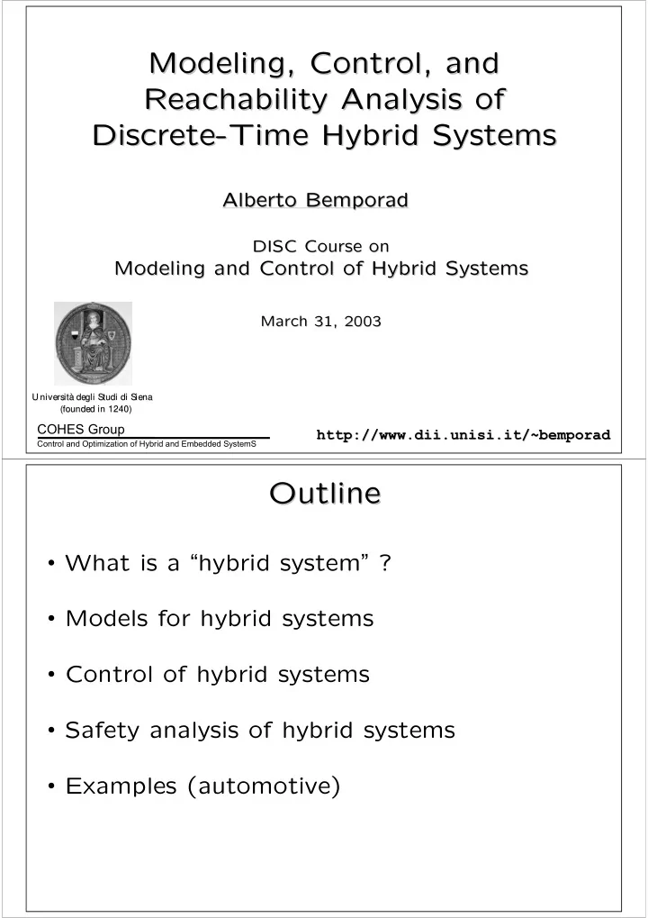
Modeling, Control, and Modeling, Control, and Reachability Reachability Analysis of Analysis of Discrete Discrete-

• Time Hybrid Systems

Time Hybrid Systems

DISC Course on DISC Course on

Modeling and Control of Hybrid Systems Modeling and Control of Hybrid Systems

March 31, 2003 March 31, 2003

Alberto Bempora Alberto Bemporad Alberto Bempora Alberto Bemporad

U niversit U niversità à degli degli Studi Studi di Siena di Siena (founded in 1240) (founded in 1240)

http:// http://www.dii.unisi.it/~bemporad www.dii.unisi.it/~bemporad

COHES Group

Control and Optimization of Hybrid and Embedded SystemS

Outline Outline

• What is a “hybrid system” ?
• Models for hybrid systems
• Control of hybrid systems
• Safety analysis of hybrid systems
• Examples (automotive)

Motivating Problem Motivating Problem

GO GOAL: command gear ratio, gas pedal, and brakes to trac track k a desired speed and minimize consumptions CHALLEN CHALLENGES: ES:

• continuous and

and discrete inputs

• dynamics depends on gear
• nonlinear torque/speed maps

Hybrid systems

Hybrid Systems Hybrid Systems

dt dx(t)

= f(x(t), u(t)) y(t) = g(x(t), u(t)) ú X = {1, 2, 3, 4, 5} U = {A, B, C}

Computer Science Control Theory Finite state machines Continuous dynamical systems system

u(t) y(t)

x ∈ Rn, u ∈ Rm y ∈ Rp

A B C C A B B C

(Witsenhausen, 1966)

continuous dynamical system

discrete inputs

Motivation: Embedded Systems Motivation: Embedded Systems

symbols symbols continuous states continuous inputs

automaton / logic interface

• Consumer electronics
• Home appliances
• Office automation
• Automobiles
• Industrial plants
• ...

Motivation: “ Motivation: “Intrisically Intrisically Hybrid” Hybrid”

• Transmission

Discrete command (R,N,1,2,3,4,5)

• Four-stroke engines

Automaton, dependent on power train motion Continuous dynamical variables (velocities, torques)

+

Key Requirements for Hybrid Models Key Requirements for Hybrid Models

• Descriptiv

Descriptive enough to capture the behavior of the system – continuous dynamics (physical laws) – logic components (switches, automata, software code) – interconnection between logic and dynamics

• Simple

Simple enough for solving analysis and synthesis problems

x0 = Ax + Bu y = Cx + Du

x0 = f(t, x, u) y = g(t, x, u)

linear systems nonlinear systems linear hybrid systems

? Piecewise Affine Systems Piecewise Affine Systems

• Approximates nonlinear dynamics arbitrarily well
• Suitable for stability analysis, reachability analysis

(verification), controller synthesis, ...

(Sontag 1981)

state+input space

Discrete Hybrid Automata Discrete Hybrid Automata

(Torrisi, Bemporad, 2003)

Switched Affine Systems Switched Affine Systems

Linear affine dynamics depends upon the mode i(k)

Event Generator Event Generator

Generates a logic signal according to the satisfaction of a linear affine constraint

Finite State Machine Finite State Machine

Discrete dynamics evolving according to a Boolean state update function

Mode Selector Mode Selector

a Boolean function selects the active mode i(k) of the SAS

Glover 1975, Williams 1977

Logic and Inequalities Logic and Inequalities

Transformation of Logic into Transformation of Logic into Linear Integer Inequalities Linear Integer Inequalities

Aî ô B, î ∈ {0, 1} V

j=1 m

W

i∈Pj Xi

W

i∈Nj X

ö i ð ñ

• 1. Convert to Conjunctive Normal Form (CNF):

1 ô X

i∈P1

îi + X

i∈N1

(1 à îi) . . . . . . . . . 1 ô X

i∈Pm

îi + X

i∈Nm

(1 à îi)

• 2. Transform into inequalities:

Every logic proposition can be translated into linear integer inequalities

• 0. Given a Boolean statement F(X1, X2, . . ., Xn)

Geometric approach: The polytope is the convex hull of the rows of the truth table

General Transformation into General Transformation into Linear Integer Inequalities Linear Integer Inequalities

Every logic proposition can be translated into linear integer inequalities P,{î : Aî ô B}

T

Aî ô B, î ∈ {0, 1}n

Truth Tables Linear Integer Truth Tables Linear Integer Inequalities Inequalities

Example: logic “AND” Convex hull algorithms: cdd, lrs, qhull, chD, Hull, Porto

3 1 2

conv " # , 1 " # , 1 " # , 1 1 1 " # ! = î : à î1 + î3 ô 0 à î2 + î3 ô 0 î1 + î2 à î3 ô 1      

Key idea: White points cannot be in the hull of black points

Mixed Logical Dynamical Systems Mixed Logical Dynamical Systems

DHA

• Computationally oriented (Mixed Integer Programming)
• Suitable for optimal controller synthesis, verification, ...

Continuous and binary variables

(Bemporad, Morari 1999)

Mixed Logical Dynamical (MLD) Systems

M = à m = 10 ï > 0 small

• Associate

A Simple Example A Simple Example

• System:
• Then
• Rewrite as linear equation

and transform x(t + 1) = 0.8x(t) + u(t) if x(t) õ 0 à 0.8x(t) + u(t) if x(t) < 0 ú

[î(t) = 1] ↔ [x(t) õ 0] x(t + 1) = 1.6î(t)x(t) à 0.8x(t) + u(t) z(t) = î(t)x(t)

à 10 ô x(t) ô 10, à 1 ô u(t) ô 1 à mî(t) ô x(t) à m à (M + ï)î(t) ô à x(t) à ï z(t) ô Mî(t) z(t) õ mî(t) z(t) ô x(t) à m(1 à î(t)) z(t) õ x(t) à M(1 à î(t)) x(t + 1) = 1.6z(t) à 0.8x(t) + u(t)

HYSDEL HYSDEL

( (HYbrid HYbrid Systems Systems DEscription DEscription Language) Language)

• Describe hybrid systems:

– Automata – Logic – Lin. Dynamics – Interfaces – Constraints

(Torrisi, Bemporad, 2003)

• Automatically generate MLD models in Matlab

ht http:/ tp://contro /control.et l.ethz.ch/~ hz.ch/~hybr hybrid/hysd id/hysdel el

• MLD model is not unique in terms of the number of auxiliary

variables optimize model (minimize # binary variables !)

SYSTEM tank { INTERFACE { STATE { REAL h [-0.3,0.3]; } INPUT { REAL Q [-10,10]; } PARAMETER { REAL k = 1; REAL e = 1e-6; } } /* end interface */ IMPLEMENTATION { AUX { BOOL s; } AD { s = hmax - h <= 0; } CONTINUOUS { h = h + k * Q; } } /* end implementation */ } /* end system */

Example 1: AD section Example 1: AD section

[ ] [ ]

max

s h h = ↔ ≥ T

Example 2: DA section Example 2: DA section

( ) 2.3 1.3 ( )

t comp t t

u u u u u u u u <  =  − ≥ 

SYSTEM motor { INTERFACE { STATE { REAL ucomp; } INPUT { REAL u [0,10]; } PARAMETER { REAL ut = 1; REAL e = 1e-6;} } /* end interface */ IMPLEMENTATION { AUX { REAL unl; BOOL th; } AD { th = ut - u <= 0; } DA { unl = { IF th THEN 2.3*u - 1.3*ut ELSE u }; } CONTINUOUS { ucomp = unl; } } /* end implementation */ } /* end system */

Nonlinear amplification unit

Example 3: LOGIC section Example 3: LOGIC section

( )

brake alarm tunnel fire

u u s s = ∧ ¬ ∨ ¬

fire alarm

s u →

SYSTEM train { INTERFACE { STATE { BOOL brake; } INPUT { BOOL alarm, tunnel, fire; } } /* end interface */ IMPLEMENTATION { AUX { BOOL decision; } LOGIC { decision = alarm & (~tunnel | ~fire); } AUTOMATA { brake = decision; } MUST { fire -> alarm; } } /* end implementation */ } /* end system */

Example 4: CONTINUOUS section Example 4: CONTINUOUS section

( ) d i C u t dt =

( 1) ( ) ( ) T u k u k i k C + = +

Apply forward difference rule:

SYSTEM capacitorD { INTERFACE { STATE { REAL u; } PARAMETER { REAL R = 1e4; REAL C = 1e-4; REAL T = 1e-1; } } /* end interface */ IMPLEMENTATION { CONTINUOUS { u = u - T/C/R*i; } } /* end implementation */ } /* end system */

Example 5: AUTOMATA section Example 5: AUTOMATA section

SYSTEM outflow { INTERFACE { STATE { BOOL closing, stop, opening; } INPUT { BOOL uclose, uopen, ustop; } } /* end of interface */ IMPLEMENTATION { AUTOMATA { closing = (uclose & closing) | (uclose & stop); stop = ustop | (uopen & closing) | (uclose & opening);

• pening = (uopen & stop) | (uopen & opening); }

MUST { ~(uclose & uopen); ~(uclose & ustop); ~(uopen & ustop); } } /* end implementation */ } /* end system */

Example 6: MUST section Example 6: MUST section

max

h h ≤ ≤

SYSTEM watertank { INTERFACE { STATE { REAL h; } INPUT { REAL Q; } PARAMETER { REAL hmax = 0.3; REAL k = 1; } } /* end interface */ IMPLEMENTATION { CONTINUOUS { h = h + k*Q; } MUST { h - hmax <= 0;

• h <= 0; }

} /* end implementation */ } /* end system */

Modeling Flow Modeling Flow

x(t + 1) = A1x(t) + B1u(t) + f1 A2x(t) + B2u(t) + f2 x(t + 1) = A3x(t) + B3u(t) + f3 x(t + 1) =

g12x(t) + h12u(t) < k12 g32x(t) + h32u(t) < k32 g23x(t) + h23u(t) < k23 g13x(t) + h13u(t) < k13

A/D D/A continuous logic

Designer Hysdel

MLD PWA HYSDEL Source

Piecewise Affine form Mixed Logical Dynamical form

Example: Bouncing Ball Example: Bouncing Ball

F= m g

x ¨ = à g x ô 0 ⇒ x ç (t+) = à (1 à ë)x ç (tà)

How to model this system in MLD form? ë ∈ [0, 1]

x N

HYSDEL HYSDEL -

• Bouncing Ball

Bouncing Ball

SYSTEM bouncing_ball { INTERFACE {

/* Description of variables and constants */

STATE { REAL height [-10,10]; REAL velocity [-100,100]; } PARAMETER { REAL g=9.8; REAL dissipation=.4; /* 0=elastic, 1=completely anelastic */ REAL Ts=.05; } } IMPLEMENTATION { AUX { REAL z1; REAL z2; BOOL negative; } AD { negative = height <= 0; } DA { z1 = { IF negative THEN height-Ts*velocity ELSE height+Ts*velocity-Ts*Ts*g}; z2 = { IF negative THEN -(1-dissipation)*velocity ELSE velocity-Ts*g}; } CONTINUOUS { height = z1; velocity=z2;} }}

System Theory for Hybrid Systems System Theory for Hybrid Systems

• Analysis

– Well-posedness – Realization & Transformation – Stability – Reachability (=Verification) – Observability

• Synthesis

– Control – State estimation – Identification – Modeling language

Well Well-

• posedness

posedness

• MLD well-posedness :

are single valued

î(t) = F(x(t), u(t)) z(t) = G(x(t), u(t)) {x(t), u(t)} → {x(t + 1)} {x(t), u(t)} → {y(t)}

Numerical test based on mixed-integer programming available

(Bemporad, Morari, Automatica, 1999)

Are state and output trajectories defined ? Uniquely defined ? Persistently defined ?

Realization and Transformation Realization and Transformation (State (State-

• Space Hybrid Models)

Space Hybrid Models)

Other Existing Hybrid Models Other Existing Hybrid Models

• Linear complementarity (LC) systems

x(t + 1) = Ax(t) + B1u(t) + B2w(t) y(t) = Cx(t) + D1u(t) + D2w(t) v(t) = E1x(t) + E2u(t) + E3w(t) + e4 0 ô v(t)⊥w(t) õ 0

Ex: mechanical systems circuits with diodes etc.

• Extended linear complementarity (ELC) systems
• Min-max-plus-scaling (MMPS) systems

M := xi|ë| max(M1, M2)| min(M1, M2)|M1 + M2|ìM1

x(t + 1) = Mx(x(t), u(t), d(t)) y(t) = My(x(t), u(t), d(t)) 0 õ Mc(x(t), u(t), d(t))

MMPS function: defined by the grammar

Generalization of LC systems

x(t + 1) = 2 max(x(t), 0) + min(à 2

1u(t), 1)

Example:

Used for modeling discrete-event systems (t=event counter)

(De Schutter, Van den Boom, 2000) (De Schutter, De Moor, 2000) (Heemels, 1999)

Equivalences of Hybrid Models Equivalences of Hybrid Models

Σ1 Σ2

x(0)=x(0) u(k) x(k), y(k) x(k), y(k)

Equivalence Results Equivalence Results

(Heemels, De Schutter, Bemporad, Automatica, 2001)

Theoretical properties and analysis/synthesis tools can be transferred from one class to another

MLD PWA MMPS ELC LC

? ? ? ? ? ? ? ?

DHA

? (Torrisi, Bemporad, IEEE CST, 2003) (Bemporad and Morari, Automatica, 1999) (Bemporad, Ferrari-T.,Morari, IEEETAC, 2000)

Efficient Efficient MLD MLD to to PWA PWA Conversion Conversion

• Proof is constructive: given an MLD system it

returns its equivalent PWA form

• Drawback: it needs the enumeration of all possible

combinations of binary states, binary inputs, and δ variables

• Most of such combinations lead to empty regions Ω
• IDEA: use techniques from multiparametric

programming to avoid such an enumeration

MLD MLD to to PWA PWA Conversion Algorithm Conversion Algorithm

Note Note: the cells Ωi are embedded in Rn+m by treating integer states and integer inputs as continuous vars: xb,ub ∈ [0,1] → xb,ub ∈ [-1/2,1/2) ∪ [1/2,3/2]

GOAL GOAL: split a given set B of states+inputs into polyhedral cells and find the affine dynamics in each cell, therefore determining the PWA system which is equivalent to the given MLD system

B

x u

(Bemporad, 2002)

Example: Heat and Cool Example: Heat and Cool

Cold air flow Hot air flow

#1 #2 T1 T2 Tamb

Rules of the Rules of the game: game:

Hybrid Hybrid HYSDEL HYSDEL Model Model Hybrid Hybrid MLD MLD Model Model

• MLD model
• 2 continuous states:
• 1 continuous input:
• 6 auxiliary binary vars:
• 2 auxiliary continuous vars:

(room temperature Tamb) (temperatures T1,T2) (water flows uhot, ucold) (4 thresholds + 2 for OR condition)

• 20 mixed-integer inequalities

Possible combination of integer variables: 26 = 64

Hybrid Hybrid PWA PWA Model Model

• PWA model
• 2 continuous states:
• 1 continuous input:

(room temperature Tamb) (temperatures T1,T2)

• 5 polyhedral regions

(partition does not depend on input)

Computation time: 0.72 s in Matlab

uhot = ¯ UH ucold = uhot = ucold = ¯ UC uhot = ucold =

• 10

10 20 30 40 50

• 10

10 20 30 40 50 Temperature T

1 (deg C)

Temperature T

2 (deg C)

Controller Synthesis Controller Synthesis

Model Predictive Control Model Predictive Control

• f Hybrid Systems
• f Hybrid Systems

y(t) u(t)

Hybrid System

Reference r(t) Output Input Measurements

Controller

• MODEL: a model of the plant is needed to predict the future

behavior of the plant

• PREDICTIVE: optimization is based on the predicted future

evolution of the plant

• CONTROL: control complex constrained multivariable plants

Receding Horizon Philosophy Receding Horizon Philosophy

• Only apply the first optimal move

Solve an optimal control problem over a finite future horizon p : – minimize – subject to constraints

Predicted outputs Manipulated Inputs t t+1 t+p

u(t+k) r(t)

t+1 t+2 t+p+1

• At time t :
• Get new measurements, and repeat the optimization

at time t +1 Advantage of on-line optimization: FEED

FEEDBACK! BACK!

|y à r| + ú|u|

umin ô u ô umax ymin ô y ô ymax

uã(t)

Receding Horizon Receding Horizon -

• Example

Example

MPC is like playing chess !

minUJ(U, x(t), r), P

k=0 Tà1

kQ(y(t + k + 1|t) à r)k + kR(u(t + k) à ur)k

• Apply only (discard the remaining optimal inputs)
• At time t

solve with respect to the finite-horizon open-loop, optimal control problem:

• subj. to

MLD model x(t|t) = x(t) x(t + T|t) = xr   

u(t) =uã(t)

MPC for Hybrid Systems MPC for Hybrid Systems

Predicted

• utputs

Manipulated y(t+k|t) Inputs t t+1 t+T

future past

u(t+k)

U,{u(t), u(t + 1). . ., u(t + T à 1)}

• Repeat the whole optimization at time t+1

+ û kî(t + k|t) à îrk + kz(t + k|t) à zrk + kx(t + k|t) à xrk ( )

Model Predictive (MPC) Control

Closed Closed-

• Loop Stability

Loop Stability

Proof: Easily follows from standard Lyapunov arguments

(Bemporad, Morari 1999)

Stability Proof Stability Proof

x(t + 1) = 0.8 cosë(t) à sinë(t) sinë(t) cosë(t) " # x(t) + 1 ô õ u(t) y(t) = 0 1 [ ] x(t) ë(t) = 3 ù if [1 0]x(t) õ 0 à 3 ù if [1 0]x(t) < 0     

Open loop: Switching System:

Hybrid MPC Hybrid MPC -

• Example

Example

Closed loop:

y(t), r(t) u(t)

time t time t

Constraint:

à 1 ô u(t) ô 1

State Estimation / Fault Detection State Estimation / Fault Detection

State Estimation / Fault Detection State Estimation / Fault Detection

• Solution: Use Moving Horizon Estimation for MLD systems (dual of MPC)

(Bemporad, Mignone, Morari, ACC 1999)

• Input disturbances
• Output disturbances

ø ∈ Rn

min P

k=1 T

y ê(t à k|t) à y(t à k) k k2 + . . .

x ê(t)

• Problem: given past output measurements and inputs, estimate the current

state/faults

MHE optimization = MIQP Convergence can be guaranteed

(Ferrari-T., Mignone, Morari, 2002)

Augment the MLD model with: At each time t solve the optimization:

ð ∈ R p

and get estimates

Fault de Fault detecti tection:

• n:

augment MLD with unknown binary binary distubances þ ∈ {0,1}p

Example: Three Tank System Example: Three Tank System

• : leak in tank 1

for

• : valve V1 blocked

for

þ1 þ2 20s ô t ô 60s t õ 40s

COSY Benchmark problem, ESF

Example: Three Tank System Example: Three Tank System

[h1 ô hv] ⇒ þ2 = 0

• Add logic constraint

COSY Benchmark problem, ESF

• : leak in tank 1

for

• : valve V1 blocked

for

þ1 þ2 20s ô t ô 60s t õ 40s

Optimal Control of Hybrid Systems: Optimal Control of Hybrid Systems: Computational Aspects Computational Aspects

min

ø

J(ø, x(t)) = 2 1ø0Hø + x 0(t)Fø + 2 1x 0(t)Yx(t) s.t.Gø ô W + Sx(t)

Mixed Integer Quadratic Program (MIQP)

• Set

MIQP Formulation of MPC MIQP Formulation of MPC

min X

k=0 Tà1 n

y0(t + k + 1|t)Qy(t + k + 1|t) + u0(t + k)Ru(t + k)

• s.t.MLD dynamics

ø,[u(t),...,u(t +Tà1),î(t|t),...,î(t +Tà1|t),z(t|t),...,z(t +Tà1|t)]

ø ∈ RT(n u+n z) â {0, 1}Tn î u ∈ Rn u î ∈ {0, 1}n î z ∈ Rn z

(Bemporad, Morari, 1999)

MILP Formulation of MPC MILP Formulation of MPC

min X

k=0 Tà1

kQy(t + k + 1|t)k∞ + kRu(t + k)k∞ s.t.MLD dynamics

min

ø

J(ø, x(t)) = X

k=0 Tà1

ïx

i + ïu i

s.t.Gø ô W + Sx(t)

Mixed Integer Linear Program (MILP)

• Set ø,[ïx

1, . . ., ïx Ny, ïu 1, . . ., ïTà1, U, î, z]

• Introduce slack variables:

ïx

k

õ [Qy(t + k|t)]i i = 1, . . ., p, k = 1, . . ., T à 1 ïx

k

õ à [Qy(t + k|t)]i i = 1, . . ., p, k = 1, . . ., T à 1 ïu

k

õ [Ru(t + k))]i i = 1, . . ., m, k = 0, . . ., T à 1 ïu

k

õ à [Ru(t + k))]i i = 1, . . ., m, k = 0, . . ., T à 1

ïx

k

õ kQy(t + k|t)k∞ ïu

k

õ kRu(t + k)k∞

min |x| min ï s.t. ï õ x ï õ à x

(Bemporad, Borrelli, Morari, 2000)

• General purpose Branch & Bound/Branch & Cut solvers available

for MILP and MIQP (Ilog CPLEX, XPRESS-MP, Sahinidis, ...)

BUT

• Mixed-Integer Programming is NP-hard

Mixed Mixed-

• Integer Program Solvers

Integer Program Solvers

Phase ase tra transiti sitions

• ns have been found in

computationally hard problems.

(Monasson et al., Nature, 1999)

• No need to reach global optimum (see proof of the theorem),

although performance deteriorates

http://plato.la.asu.edu/bench.html

More solvers and benchmarks:

0 2

3 4 5

Ratio of Constraints to Variables

6 7 8 1000 3000

Cost of Computation

2000 4000

50 var 40 var 20 var

… but not for fast sampling (e.g. 10 ms) / cheap hardware ! Good for large sampling times (e.g., 1 h) / expensive hardware …

Hybrid Control Example: Hybrid Control Example: Heat Exchange Heat Exchange

Amount of heating power u is constant

(Hedlund and Rantzer, CDC1999) Bi = 1 ô õ if first furnace heated 1 ô õ if second furnace heated ô õ if no heating               

• Objective:
• Control the temperature

to a given set-point

• Constraints:
• Only three operation modes:

1- Heat only the first furnace 2- Heat only the second furnace 3- Do not heat any furnaces T ç1 T ç2 ô õ = à 1 à 2 ô õ T1 T2 ô õ + Biu0 T1, T2

Hybrid Control Hybrid Control -

• An Example

An Example

Alternate Heating of Two Furnaces Alternate Heating of Two Furnaces

• HYSDEL model:

x(t + 1) = h 0.9231

0.8521 1.0000

i x(t) + h 1 0

0 1 0 0

i z(t)      

−1 1 −1 1 −1 1 −1 1

      z(t)      

−0.7688 0.7688 −0.7393 0.7393 −1.0000 −1.0000

      u(t) +     

−0.0769 0.0769 −0.0739 0.0739

     x3(t) +     

0.7688 0.7393 1.0000

    

• MLD model:

• Performance index

min u(t),u(t+1),u(t+2)

{ }

P

k=0 2

kR(u(t +k +1) àu(t +k))k∞+kQ(x(t +k|t) àxe)k∞

à 1 ô x1 ô 1 à 1 ô x2 ô 1

Alternate Heating of Two Furnaces Alternate Heating of Two Furnaces

• Constraints

Closed Closed-

• Loop Behavior

Loop Behavior

u0=0.8

X1 X2 X1 X2

u0=0.4

Set point cannot be reached Set point is reached

• Computational complexity
• f on-line MILP

Linear constraints Continuous variables Binary variables Parameters Time to solve MILP (av.) 168 33 6 3 1,09 s

(Bemporad, Borrelli, Morari, 2000)

On On-

• Line vs. Off

Line vs. Off-

• Line Optimization

Line Optimization

• On-line optimization: given x(t), solve the problem at each time step t

multi-parame multi-parametric Mixed Intege tric Mixed Integer Line r Linear Progr ar Program ( am (mp-MILP) p-MILP) Mixed-Integer Linear Program (MILP)

• Off-line optimization: solve the MILP fo

for a r all x(t)

minUJ(U, x(t)), P

k=0 Tà1

kQy(t + k + 1|t)k∞ + kRu(t + k)k∞

• subj. to

MLD model x(t|t) = x(t) x(t + T|t) = 0    min

ø

J(ø, x(t)),f 0ø s.t.Gø ô W + Fx(t)

Explicit Form of Explicit Form of Model Predictive Control Model Predictive Control via via Multiparametric Multiparametric Programming Programming

• 60
• 40
• 20

20 40 60

• 60
• 40
• 20

20 40 60

CR{2,3} CR{1,4} CR{1,2,3} CR{1,3} x1 x2

Example of Example of Multiparametric Multiparametric Solution Solution

Multiparametric LP ( )

ø ∈ R2

• Linear Model:

x(t + 1) = Ax(t) + Bu(t) y(t) = Cx(t)

Linear MPC Linear MPC

y(t + k|t) = CAkx(t) + P

i=0 kà1 CAiBu(t + k à 1 à i)

u(t + k) = u(t à 1) + P

i=0 kà1 ∆u(t + i)

• Prediction:

∆u(t) = u(t) à u(t à 1)

input increments (for integral action)

Linear MPC Linear MPC

minUJ(U, x(t)) = 2

1U0HU + [x0(t) r0(t)]FU + 2 1[x0(t) r0(t)]Y

x(t) r(t) ô õ

(convex) QU QUADRA RATIC TIC PROGRAM PROGRAM (QP) (QP)

subject to GU ô W + K x(t) r(t) ô õ Constraints

U,{∆u(t),.. ., ∆u(t +m à1)}

minU P

k=0 pà1 kWy y(t + k + 1|t) à r(t)

[ ] k2

ymin ô y(t + k|t) ô ymax, k = 1, . . ., p umin ô u(t + k) ô umax, k = 0, 1, . . ., m à 1 ∆umin ô ∆u(t + k) ô ∆umax, k = 0, 1, . . ., m à 1 Quadratic Performance Index

+ kW∆u∆u(t + k)k2 + Wu u(t + k) à utarget(t) [ ] k2

Multiparametric Multiparametric Quadratic Programming Quadratic Programming

• Objective: solve the QP fo

for all r all

(Bemporad et al., 2002)

Linearity of the Solution Linearity of the Solution

From (1) :

In some neighborhood of x0, λ and U are explicit affine functions of x !

solve QP to find identify active constraints at KKT

• ptimality

conditions: From (2) : form matrices by collecting active constraints x0∈ X

Determining a Critical Region Determining a Critical Region

• Impose primal and dual feasibility:
• Remove redundant constraints

critical region CR0 CR0 = {Ax ô B} CR0

x-space x0

• X
• is the set of all and only parameters x for which

is the optimal combination of active constraints at the optimizer

G à , W à , S à CR0

linear inequalities in x !

Multiparametric Multiparametric QP QP

CR0 = {Ax ô B} Ri = {x ∈ X : Aix > Bi, Ajz ô Bj, ∀j < i}

Theore Theorem: is a partition of

{CR0, R1, . . ., RN}

X ò Rn

CR0

x-space x0

• R1

R2 RN R3 X R4

Proceed iteratively: for each region repeat the whole procedure with X ←Ri

R

i

The recursive algorithm terminates after a finite number of steps, because the number of combinations

• f active constraints is finite

The active set of a neighboring region is found by using the active set of the current region + knowledge of the type of hyperplane we are crossing:

⇒ The corresponding constraint is added added to the active set ⇒ The corresponding constraint is wit withdraw drawn from the active set

CR CR CR x1 x2 x1 x2 x1 x2

Mp Mp-

• QP

QP – – More efficient method More efficient method

(Tøndel, Johansen, Bemporad, 2003)

Multiparametric Multiparametric QP QP

continuous, piecewise affine convex, continuous, piecewise quadratic, C1 (if no degeneracy) Co Coro rollary llary: The linear MPC controller is a continuous piecewise affine function of the state

Complexity Reduction Complexity Reduction

Regions where the first component of the solution is the same can be joined (when their union is convex). (Bemporad, Fukuda, Torrisi,

Computational Geometry, 2001)

U(x(0)),[u 0(x(0)), . . ., u Tà1(x(0))]

• 2.5
• 2
• 1.5
• 1
• 0.5

0.5 1 1.5 2 2.5

• 2.5
• 2
• 1.5
• 1
• 0.5

0.5 1 1.5 2 2.5 CR1 CR2 CR3 CR4 CR5 CR6 CR7 CR8 CR9

• 2.5
• 2
• 1.5
• 1
• 0.5

0.5 1 1.5 2 2.5

• 2.5
• 2
• 1.5
• 1
• 0.5

0.5 1 1.5 2 2.5 CR1 CR2 CR3 CR4 CR5 CR6 CR7

Double Integrator Example Double Integrator Example

y(t) = s2

1 u(t)

x(t + 1) = 1 1 1 ô õ x(t) + 1 ô õ u(t) y(t) = 1 [ ] x(t)

• System:

à 1 ô u(t) ô 1

• Constraints:
• Control objective: minimize

P

t=0 ∞ y0(t)y(t) + 100 1 u2(t)

ut+k = KLQ x(t + k|t) ∀k õ Nu

• Optimization problem: for Nu=2

sampling + ZOH T=1 s (cost function is normalized by max λ(H))

mp mp-

• QP solution

QP solution

Nu=2

Complexity Complexity

Nu=3 Nu=4 Nu=5 Nu=6

5 10 15 20 20 40 CPU time 5 10 15 20 100 200 300 # Regions # free moves

Extensions Extensions

• Tracking of reference r(t) :
• Rejection of measured

disturbance v(t) :

• Soft constraints:
• Variable constraints:

îu(t) = F(x(t), u(t à 1), r(t)) îu(t) = F(x(t), u(t à 1), v(t)) u(t) = F(x(t), umin(t), . . ., ymax(t)) u(t) = F(x(t)) ymin à ï ô y(t + k|t) ô ymax + ï umin(t) ô u(t + k) ô umax(t) ymin(t) ô y(t + k|t) ô ymax(t)

• Linear norms: minUJ(U, x(t)), P

k=0 p

kQy(t + k|t)k∞ + kRu(t + k)k∞

(Bemporad, Borrelli, Morari, IEEE TAC, 2002)

Closed Closed-

• Loop MPC and Hybrid Systems

Loop MPC and Hybrid Systems

Motivation: Use hybrid techniques to analyze closed-loop MPC systems !

(Bemporad, Heemels, De Schutter IEEE TAC, 2002)

DHA DHA

MPC Regulation of a Ball on a Plate MPC Regulation of a Ball on a Plate

• Tune an MPC

controller by simulation, using the MPC Simu MPC Simuli link Too Toolbox box

• Get the explic

explicit it solution solution of the MPC controller.

• Validate the

controller on experiments experiments. Ta Task sk:

B&P Experimental Setup B&P Experimental Setup

Ball & Ball & Plate Plate System System

Host Target Ball & Plate Code Data

u1, u2 a,b x, y

TCP/IP

Ball&Plate Experiment Ball&Plate Experiment

• Specifications:

Angle:

• 17 deg … +17deg

Plate:

• 30 cm …+30 cm

Input Voltage: -10 V… +10 V Computer: PENTIUM166 Sampling Time:30 ms

• Model:

LTI 14 states Constraints on inputs and states

y α β x

α' β' δ γ

E.g: MPC Toolbox for Matlab

• Step 1: Tune the MPC controller (in simulation)

General Philosophy: (1) MPC Design General Philosophy: (1) MPC Design

(Bemporad, Morari, Ricker, 2003)

General Philosophy: (2) Implementation General Philosophy: (2) Implementation

• Step 2: Solve mp-QP and implement Explicit

MPC E.g: Real-Time Workshop + xPC Toolbox

Explicit MPC Solution Explicit MPC Solution

x-MPC:

• MPC: sections at αx=0, αx=0, ux=0, rx=18, rα=0

Region 1: Region 1: Region 6: Region 6: Region 16: Region 16:

Saturation at -10 Saturation at +10 LQR Controller (near Equilibrium)

6 1 16 16 6 16 16

1

• x: 22 Regions, y: 23 Regions

Controll Controller: er:

MPC Regulation of a Ball on a Plate MPC Regulation of a Ball on a Plate

• Tune an MPC

controller by simulation, using the MPC MPC Simulink nk T Tool

• lbox

.

• Get the explic

explicit it solution solution of the MPC controller. Validate the controller on experiments experiments. Design Ste Design Steps: s:

Comments on Explicit MPC Comments on Explicit MPC

• Multiparametric Quadratic Programs (mp-QP) can be solved efficiently
• Explicit solution of MPC controlleru = f(x) is Piecewise Affine

Eliminate heav iminate heavy on-line computat y on-line computation for MP ion for MPC Make MP Make MPC C suitable suitable for fa for fast/ st/small/c mall/chea heap processes processes

• Model Predictive Control (MPC) can be solved off-line via mp-QP

MILP Formulation of MPC MILP Formulation of MPC

min X

k=0 Tà1

kQy(t + k + 1|t)k∞ + kRu(t + k)k∞ s.t.MLD dynamics

min

ø

J(ø, x(t)) = X

k=0 Tà1

ïx

i + ïu i

s.t.Gø ô W + Sx(t)

Mixed Integer Linear Program (MILP)

• Set ø,[ïx

1, . . ., ïx Ny, ïu 1, . . ., ïTà1, U, î, z]

• Introduce slack variables:

ïx

k

õ [Qy(t + k|t)]i i = 1, . . ., p, k = 1, . . ., T à 1 ïx

k

õ à [Qy(t + k|t)]i i = 1, . . ., p, k = 1, . . ., T à 1 ïu

k

õ [Ru(t + k))]i i = 1, . . ., m, k = 0, . . ., T à 1 ïu

k

õ à [Ru(t + k))]i i = 1, . . ., m, k = 0, . . ., T à 1

ïx

k

õ kQy(t + k|t)k∞ ïu

k

õ kRu(t + k)k∞

min |x| min ï s.t. ï õ x ï õ à x

(Bemporad, Borrelli, Morari, 2000)

• Theorem:

Theorem: The multiparametric solution is piecewise affine

s.t. Gøc + Eød ô W + Fx

min ø={øc,ød} f0øc + d0ød

(Dua, Pistikopoulos, 1999)

øc ∈ Rn ød ∈ {0, 1}m

• mp-MILP can be solved (by alternating MILPs and mp-LPs)

Multiparametric Multiparametric MILP MILP

• Corol

Corollary ry: The MPC controller is The MPC controller is piecew piecewise affine ise affine in in x

øã(x)

• Explicit solutions to finite-time optimal control

problems for PWA systems can be obtained using a combination of

• Dynamic Programming
• Multiparametric Linear (1-norm, ∞-norm), or
• r Quadratic (squared 2-norm) programming

Solutions via Dynamic Programming Solutions via Dynamic Programming

(Borrelli, Bemporad, Baotic, Morari, 2003) (Mayne, ECC 2001)

Note: in the 2-norm case, the partition may not be polyhedral

Hybrid Control Examples Hybrid Control Examples (Revisited) (Revisited)

x(t + 1) = 0.8 cosë(t) à sinë(t) sinë(t) cosë(t) " # x(t) + 1 ô õ u(t) y(t) = 0 1 [ ] x(t) ë(t) = 3 ù if [1 0]x(t) õ 0 à 3 ù if [1 0]x(t) < 0     

Open loop: Closed loop: Switching System:

Hybrid Control Hybrid Control -

• Example

Example

y(t), r(t) u(t)

time t time t

Constraint: à 1 ô u(t) ô 1

• MLD system
• mp-MILP optimization problem

to be solved in the region

• Computational complexity of mp-MILP

min

v

1

n oJ(v1

0,x(t)),P k=0 1

kQ1(v(k) àue)k∞ +kQ2(î(k|t) àîe)k∞ +kQ3(z(k|t) àze)k∞ +kQ4(x(k|t) àxe)k∞

subject to constraints

à 5 ô x1 ô 5 à 5 ô x2 ô 5

Hybrid MPC Hybrid MPC -

• Example

Example

Linear constraints Continuous variables Binary variables Parameters Time to solve mp-MILP Number of regions 84 20 2 2 3 min 7

State x(t) 2 variables Input u(t) 1 variables

• Aux. binary vector δ(t)

1 variables

• Aux. continuous vector z(t)

4 variables

mp mp-

• MILP Solution

MILP Solution

PWA law MPC law A law MPC law PWA law MPC law A law MPC law

ñ

Prediction Horizon T=2

Linear constraints Continuous variables Binary variables Parameters Time to solve mp-MILP Number of regions 84 20 2 2 3 min 7

mp mp-

• MILP Solution

MILP Solution

Prediction Horizon T=3 Prediction Horizon T=4

X1 X2 X1 X2

• mp-MILP optimization problem

min u(t),u(t+1),u(t+2)

{ }

P

k=0 2

kR(u(t +k +1) àu(t +k))k∞+kQ(x(t +k|t) àxe)k∞

à 1 ô x1 ô 1 à 1 ô x2 ô 1 ô u0 ô 1

Alternate Heating of Two Furnaces Alternate Heating of Two Furnaces

parameterized !

• Parameter set
• Computational complexity
• f mp-MILP

Linear constraints Continuous variables Binary variables Parameters Time to solve mp-MILP Number of regions 168 33 6 3 5 min 105

(Bemporad, Borrelli, Morari, 2000)

T1 T

2

Heat 2 No Heat

mp mp-

• MILP Solution

MILP Solution

u0=0.8

T1 T2

Heat 1 Heat 2 No Heat

X1 X2 X1 X2

u0=0.4

Set point cannot be reached Set point is reached

Heat 1

NOTE: The control action of explicit and of implicit MPC are totally equal !

Hybrid Control Example: Hybrid Control Example: Traction Control System Traction Control System

Controll Controller er suitable for real-time implementation Improve driver’s ability to control a vehicle under adverse external conditions (wet or icy roads)

MLD hybrid framework + optimization-based control strategy

Vehicle Traction Control Vehicle Traction Control

Model Model nonlinear, uncertain, constraints

Simple Traction Model Simple Traction Model

• Tire torque τt is a function of

slip ∆ω and road surface adhesion coefficient µ

ω ç e = Je 1 üc à beωe à gr üt ò ó v çv = mvrt üt ∆ω = gr ωe à rt vv

• Mechanical system
• Manifold/fueling dynamics

üc = biüd(t à üf)

∆ω Wheel slip

Lateral Force Tire Forces Tire Slip Maximum Acceleration Longitudinal Force Slip Target Zone Maximum Cornering Maximum Braking

Lateral Force Longitudinal Force Steer Angle

Tire Force Characteristics Tire Force Characteristics Hybrid Model Hybrid Model

Torque

Mixed-Logical Dynamical (MLD) Hybrid Model (discrete time)

Slip Torque µ

PWA Approximation

µ Slip

HYSDEL HYSDEL

(Hybr ybrid Syst d Systems ems Descri Descripti ption Language

• n Language)

Nonlinear tire torque τt =f(∆ω , µ)

(PWL Toolbox, Julian, 1999)

MLD Model MLD Model

State x(t) 9 variables Input u(t) 1 variable

• Aux. Binary

vars δ(t ) 3 variables

• Aux. Continuous vars z(t)

4 variables

The MLD matrices are automatically generated in Matlab format by HYSDEL

Performance and Constraints Performance and Constraints

minP

k=0 N

∆ω(k|t) à ∆ωdes | |

• Control objective:
• Constraints:
• Limits on the engine torque: à 20Nm ô üd ô 176Nm
• subj. to. MLD Dynamics
• Logic Constraint:
• Hysteresis

Experimental Apparatus Experimental Apparatus Experimental Apparatus Experimental Apparatus

Wheel Speeds, [rad/s] 20 15 10 5 25 15 12 9 6 3 18 Engine Torque Command, [Nm] 40 20

• 20

60 Time, [s] 15 12 9 6 3 18 Controller Region 25 20 15 10 5 30

Experimental Results Experimental Results

Experiment Experiment

• >500 regions
• 20ms sampling time
• Pentium 266Mhz +

Labview

Hybrid Control Example: Hybrid Control Example: Cruise Control System Cruise Control System Hybrid Control Problem Hybrid Control Problem

Renault Clio 1.9 DTI RXE GOAL: command gear ratio, gas pedal, and brakes to track a desired speed and minimize consumption

Hybrid Model Hybrid Model

ω =

ks Rg(i)x

ç mx ¨ = Fe à Fb à ìx ç Fe =

ks Rg(i)M

• Vehicle dynamics
• Transmission kinematics

discretized with sampling time Ts = 0.5 s

= engine torque = engine speed = gear

ω M i

= vehicle speed

x ç

= brake force

Fb

= traction force

Fe

Hybrid Model Hybrid Model

1000 2000 3000 4000 60 80 100 120 140 160 180

C+

e (ω)

• Max engine torque

Piecewise-linearization:

(PWL Toolbox, Julián, 1999)

http://www.renault.fr

Cà

e (ω) = ë1 + ì1ω

• Min engine torque

requires: 4 binary aux variables 4 continuous aux variables

à Cà

e (ω) ô M ô C+ e (ω)

• Engine torque

Hybrid Model Hybrid Model

ω =

ks Rg(i)x

ç Fe =

ks Rg(i)M

• Gear selection (traction force):

Fe = FeR + Fe1 + Fe2 + Fe3 + Fe4 + Fe5

depends on gear #i define auxiliary continuous variables: similarly, also requires 6 auxiliary continuous variables

• Gear selection (engine/vehicle speed):
• Gear selection:

gi ∈ {0, 1}

for each gear #i, define a binary input

IF gi = 1 THEN Fei =

ks Rg(i)M ELSE 0

Hybrid Model Hybrid Model

• MLD model

x(t + 1) = Ax(t) + B1u(t) y(t) = Cx(t) + D1u(t) + B2î(t) + B3z(t) + D2î(t) + D3z(t) E2î(t) + E3z(t) ô E4x(t) + E1u(t) + E5

• 2 continuous states:
• 2 continuous inputs:
• 6 binary inputs:
• 1 continuous output:
• 4 auxiliary binary vars:
• 16 auxiliary continuous vars:

(engine torque, brake force) (vehicle speed) (gears)

v M, Fb gR, g1, g2, g3, g4, g5

(vehicle position and speed)

x, v

(6 traction force, 6 engine speed, 4 PWL max engine torque) (PWL max engine torque breakpoints)

• 96 mixed-integer inequalities

Hysdel Hysdel Model Model

http://control.ethz.ch/~hybrid/hysdel

Hybrid Controller Hybrid Controller

• Max-speed controller

maxutJ(ut, x(t)),v(t + 1|t)

• subj. to

MLD model x(t|t) = x(t) ú MILP optimization problem ( is irrelevant) x(t) v(t) x(t)

50 100 150 200 250

Linear constraints Continuous variables Binary variables Parameters Time to solve mp-MILP (Sun Ultra 10) Number of regions 96 18 10 1 45 s 11

Hybrid Controller Hybrid Controller

• Max-speed controller

50 100 50 100 150 200 Velocity (km/h) 50 100 1000 2000 3000 4000 5000 6000 Engine speed (rpm) Time (s) 50 100 50 100 150 200 Engine Torque (Nm) Time (s) 50 100 1 2 3 4 5 Gear 50 100 10 20 30 40 50 60 Power (kW) Time (s) 50 100

• 1
• 0.5

0.5 1 Fraction of Max Torque (Nm) 50 100

• 1
• 0.5

0.5 1 Road Slope (deg) Time (s) 50 100

• 1
• 0.5

0.5 1 Brakes (Nm)

Hybrid Controller Hybrid Controller

• Tracking controller

minutJ(ut, x(t)),|v(t + 1|t) à vd(t)| + ú|ω|

• subj. to

MLD model x(t|t) = x(t) ú v(t) vd(t)

40 80 120 160 200 50 100 150 200 250

MILP optimization problem

Linear constraints Continuous variables Binary variables Parameters Time to solve mp-MILP (Sun Ultra 10) Number of regions 98 19 10 2 27 m 49

Hybrid Controller Hybrid Controller

• Tracking controller

100 200 20 40 60 80 100 120 Velocity (km/h), Desired velocity (km/h) 100 200 1000 2000 3000 4000 5000 6000 Engine speed (rpm) Time (s) 100 200

• 200
• 100

100 200 Engine Torque (Nm) Time (s) 100 200 1 2 3 4 5 Gear 100 200

• 100
• 50

50 100 Power (kW) Time (s) 100 200

• 1
• 0.5

0.5 1 Fraction of Max Torque (Nm) 100 200

• 6
• 4
• 2

2 4 6 Road Slope (deg) Time (s) 100 200 2000 4000 6000 8000 10000 Brakes (Nm)

minutJ(ut, x(t)),|v(t + 1|t) à vd(t)| + ú|ω|

ú = 0.001

Hybrid Controller Hybrid Controller

• Smoother tracking controller

minutJ(ut, x(t)),|v(t + 1|t) à vd(t)| + ú|ω|

• subj. to

|v(t + 1|t) à v(t)| < Tsamax MLD model x(t|t) = x(t)    v(t) vd(t)

40 80 120 160 200 50 100 150 200 250

MILP optimization problem

Linear constraints Continuous variables Binary variables Parameters Time to solve mp-MILP (Sun Ultra 10) Number of regions 100 19 10 2 28 m 54

Hybrid Controller Hybrid Controller

• Smoother tracking controller

100 200 20 40 60 80 100 120 Velocity (km/h), Desired velocity (km/h) 100 200 1000 2000 3000 4000 5000 6000 Engine speed (rpm) Time (s) 100 200

• 200
• 100

100 200 Engine Torque (Nm) Time (s) 100 200 1 2 3 4 5 Gear 100 200

• 100
• 50

50 100 Power (kW) Time (s) 100 200

• 1
• 0.5

0.5 1 Fraction of Max Torque (Nm) 100 200

• 6
• 4
• 2

2 4 6 Road Slope (deg) Time (s) 100 200 2000 4000 6000 8000 10000 Brakes (Nm)

Reachability Reachability Analysis Analysis (Verification) (Verification)

Verification Verification

• GI

GIVEN VEN: an embedded system (continuous dynamical system + logic controller)

• CERTIFY

CERTIFY that such combination behaves as desired

• for ALL initial conditions within a given set
• for ALL disturbances within a given class
• or PRO

PROVID VIDE E a counterexample.

Simulation: provides a partial answer (not all possibilities can be tested!) Reachability Analysis: provides the answer.

Ariane Ariane 5 5 -

• 1996

1996

4 5

For 1=1:10 a[i]=0; end while (x) read file For 1=1:10 a[i]=0; end while (x) read file For 1=1:10 a[i]=0; end …

4

For 1=1:10 a[i]=0; end while (x) read file For 1=1:10 a[i]=0; end while (x) read file For 1=1:10 a[i]=0; end …

4

+ + + +

Physical Physical beaviour beaviour Computer code Computer code

Need for verification Need for verification

• Success

Success

• Failure

Failure

• If yes, from which subset of ?
• Disturbance/input sequences driving to .
• Target sets (disjoint)
• A hybrid system

X(0) Σ

Reachability Reachability Analysis/Verification Analysis/Verification

• Given:

Z1, Z2, . . ., ZL t ô Tmax

• Problem:• Is reachable from in t steps ?

Zi X(0) X(0) Zi XZi(0) XZi(0)

• A set of initial conditions
• Time horizon

Z1 Z2 ZL

XZ1(0) XZ2(0) XZL(0)

X(0)

(Bemporad, Torrisi, Morari, 2000)

Applications Applications

• Safety ( = unsafe sets)
• Stability ( = invariant set around the origin)
• Optimal control ( = optimal strategy,

= reference set)

• (practical) Liveness ( = set to be reached within a finite

time)

• Robust Simulation

Z1, Z2, . . ., ZL Z1

u(0), . . ., u(Tmax)

Z1 Z1

XZ1(0) XZ2(0) XZ L(0)

Z1 Z2 ZL X(0)

(Bemporad, Giovanardi, Torrisi, CDC 2000)

Verification Algorithm via Verification Algorithm via MILP MILP

• Only practical for small problems ! because number of free

integer variables grows with T

• Efficient Solution

Efficient Solution: Exploit the special structure of the problem.

î(0), î(1), . . ., î(T)

• Simple solution: Solve ∀T>0 the mixed-integer linear feasibility test

x(0) ∈ X(0) x(T) ∈ Zi u(t) ∈ U, 0 ô t ô T x(t + 1) = Ax(t) + B1u(t) + B2î(t) + B3z(t) E2î(t) + E3z(t) ô E1u(t) + E4x(t) + E5          x(0), {u(t), î(t), z(t)}T

t=0

with respect to

(Bemporad, Torrisi, Morari, 2000) (Torrisi, Bemporad, Giovanardi, 2003)

Reach Reach-

• Set Evolution

Set Evolution

(Bemporad, Torrisi, Morari, 2000)

– Compute the polyhedral reach set X(t) – Detect switching – Describe new intersections X(t) ∩ Cj – Stopping criteria for a single exploration – Organize the search

Ci Cj Tmax < ∞, discrete-time ⇒ Decidable but NP-hard

X(0) X(1) X(2) X(3) X(4)

Reachability analysis algorithm:

Reach set implicitly defined by linear inequalities

Reach Set Computation Reach Set Computation

• Simple to compute
• Number of constraints grows linearly with time
• Explicit form also possible via projection

methods (e.g. CDD, Fukuda 1997) where is the current region

Approximation of Intersections Approximation of Intersections

Simple to compute via Linear Programming (LP) Can approximate with arbitrary precision Trade off between conservativeness and complexity Both inner and outer approximations in one shot Approximate computation of projections

Stopping Criteria Stopping Criteria

• Reach set has left the current region
• Reach set is all inside a target Zi
• t > Tmax (to guarantee termination)

X (5, X (0)) X (0) X (1, X (0)) X (2, X (0)) X (3, X (0)) X (4, X (0))

C1 C2 X (0) X (1, X (0)) X (2, X (0)) X (3, X (0))

Zi

Graph of Evolution Graph of Evolution

• The graph is initialized with all the initial subsets

Xi=X(0)∩ Ci and all the target sets

• A node is added for each initial region of a new

exploration

• If a set can reach another set, an oriented arc is

drawn

• The time needed to reach the set is a weight

associated with the arc

3

Z

X

1

X

2

2

Z

1

1 1 1

2 2

3 3 4 4

• Less conservative
• Graph more complicate

LP determines if a switching sequence is feasible

Conservativeness Conservativeness vs vs Graph Complexity Graph Complexity

• Graph less complicate
• More conservative

Verification Example: Verification Example: Cruise Control System Cruise Control System

Cruise Control System Cruise Control System

GO GOAL: Verify if a given switching controller satisfies certain specifications

(Torrisi, Bemporad, 2001)

Cruise Control System Cruise Control System

Gear selector: Speed controller:

Verification Problem Verification Problem

2 4 6 8 10 12 14 16 20 40 60 80 100 120

Time (s) Speed (Km/h)

Liveness Safety

Question: Will the cruise control reach the desired speed reference within 10 s without exceeding the speed limit? Liveness Safety

SYSTEM car { INTERFACE { STATE { REAL speed, err, vr; BOOL gear1, gear2, gear3, gear4, gear5; } PARAMETER {…}} IMPLEMENTATION { AUX { REAL Fe1, Fe2, Fe3, Fe4, Fe5, w1, w2, w3, w4, w5, DCe1, DCe2, DCe3, DCe4,zut, zub, ierr, torque, F_brake; BOOL dPWL1, dPWL2, dPWL3, dPWL4, sd, su, verr, sat_torque, sat_F_brake, no_sat;} LOGIC { no_sat = ~(sat_torque | sat_F_brake) & verr; } AD {dPWL1 = wPWL1 - (w1 + w2 + w3 + w4 + w5) <= 0; dPWL2 = wPWL2 - (w1 + w2 + w3 + w4 + w5) <= 0; dPWL3 = wPWL3 - (w1 + w2 + w3 + w4 + w5) <= 0; dPWL4 = wPWL4 - (w1 + w2 + w3 + w4 + w5) <= 0; sd = (w1 + w2 + w3 + w4 + w5) - wl <= 0; su = wu - (w1 + w2 + w3 + w4 + w5) <= 0; verr = speed - vr - 2 <= 0; sat_torque = - zut + (DCe1 + DCe2 + DCe3 + DCe4) + 1 <= 0; sat_F_brake = - zub + max_brake_force <= 0; } DA {Fe1 = {IF gear1 THEN torque / speed_factor * Rgear1}; Fe2 = {IF gear2 THEN torque / speed_factor * Rgear2}; Fe3 = {IF gear3 THEN torque / speed_factor * Rgear3}; Fe4 = {IF gear4 THEN torque / speed_factor * Rgear4}; Fe5 = {IF gear5 THEN torque / speed_factor * Rgear5}; w1 = {IF gear1 THEN speed / speed_factor * Rgear1}; w2 = {IF gear2 THEN speed / speed_factor * Rgear2}; w3 = {IF gear3 THEN speed / speed_factor * Rgear3}; w4 = {IF gear4 THEN speed / speed_factor * Rgear4}; w5 = {IF gear5 THEN speed / speed_factor * Rgear5}; DCe1 = {IF dPWL1 THEN (aPWL2) + (bPWL2) * (w1 + w2 + w3 + w4 + w5) ELSE (aPWL1) + (bPWL1) * (w1 + w2 + w3 + w4 + w5)}; DCe2 = {IF dPWL2 THEN (aPWL3 - aPWL2) + (bPWL3 - bPWL2) * (w1 + w2 + w3 + w4 + w5)}; DCe3 = {IF dPWL3 THEN (aPWL4 - aPWL3) + (bPWL4 - bPWL3) * (w1 + w2 + w3 + w4 + w5)}; DCe4 = {IF dPWL4 THEN (aPWL5 - aPWL4) + (bPWL5 - bPWL4) * (w1 + w2 + w3 + w4 + w5)}; zut = {IF verr THEN kt * (vr - speed) + it * err}; zub = {IF ~verr THEN - kb * (vr - speed) - ib * err}; torque ={IF sat_torque THEN (DCe1 + DCe2 + DCe3 + DCe4) + 1 ELSE zut}; F_brake = {IF sat_F_brake THEN max_brake_force ELSE zub}; ierr = {IF no_sat THEN err + Ts * (vr - speed)};} CONTINUOUS { speed = speed + Ts / mass * (Fe1 + Fe2 + Fe3 + Fe4 + Fe5 - F_brake - beta_friction * speed); err = ierr; vr = vr;} AUTOMATA { gear1 = (gear2 & sd) | (gear1 & ~su); gear2 = (gear1 & su) | (gear3 & sd) | (gear2 & ~sd & ~su); gear3 = (gear2 & su) | (gear4 & sd) | (gear3 & ~sd & ~su); gear4 = (gear3 & su) | (gear5 & sd) | (gear4 & ~sd & ~su); gear5 = (gear4 & su) | (gear5 & ~sd );} MUST {

• w1 <= -wemin; w1 <= wemax; -w2 <= -wemin; w2 <= wemax; -w3 <= -wemin; w3 <= wemax; -w4 <= -wemin; w4 <= wemax; -w5 <= -wemin;

w5 <= wemax; -F_brake <= 0; F_brake <= max_brake_force; torque - (DCe1 + DCe2 + DCe3 + DCe4) - 1 <= 0;

• ((REAL gear1) + (REAL gear2) + (REAL gear3) + (REAL gear4) + (REAL gear5)) <= -0.9999;

(REAL gear1) + (REAL gear2) + (REAL gear3) + (REAL gear4) + (REAL gear5) <= 1.0001; dPWL4 -> dPWL3; dPWL4 -> dPWL2; dPWL4 -> dPWL1; dPWL3 -> dPWL2; dPWL3 -> dPWL1; dPWL2 -> dPWL1;}}

Hysdel Hysdel Model Model (

(HYbrid HYbrid Systems Systems DEscription DEscription Language) Language)

Hybrid Model Hybrid Model

• MLD model
• 3 continuous states:
• 5 binary states:
• 15 auxiliary binary vars:
• 19 auxiliary continuous vars:

(gears)

g1, g2, g3, g4, g5

(speed, reference and tracking error)

v, vr, e

(5 traction force, 5 engine speed, 5 reset/saturation, 4 PWL max engine torque) (4 PWL max torque breakpoints, 4 saturations 5 logic updates, 2 gear switching conditions)

• 173 mixed-integer inequalities
• For

the verification algorithm finds the first counterexample after ˜7m

• For all the controller

satisfies both liveness & safety properties

• CPU time: ˜2.5h (Matlab 5.3, PC650MHz)

Verification Results Verification Results

vr ∈

2 4 6 8 10 12 14 16 20 40 60 80 100 120

Time (s) Speed (Km/h)

Liveness Safety

[30,120] km/h vr ∈ [30,70] km/h

Conclusions Conclusions

• Hybrid sy

Hybrid system stems as a framework for new applications, where both logic and continuous dynamics are relevant

• Mixed Logic

Mixed Logical Dy l Dynamical ( namical (MLD) systems as discrete- time, computation-oriented models for hybrid systems

x(t + 1) = Ax(t) + B1u(t) y(t) = Cx(t) + D1u(t) + B2î(t) + B3z(t) + D2î(t) + D3z(t) E2î(t) + E3z(t) ô E4x(t) + E1u(t) + E5

HYSDEL

Conclusions Conclusions

• Hybrid sy

Hybrid system stems as a framework for new applications, where both logic and continuous dynamics are relevant

• Mixed Logic

Mixed Logical Dy l Dynamical ( namical (MLD) systems as discrete- time, computation-oriented models for hybrid systems

y(t) u(t) Plant Output Input Measurements

• Piecewise Line

Piecewise Linear ar Optimal Controllers timal Controllers can be synthesized via off-line multiparametric programming for fast-sampling applications

• Supervisory MPC c

Supervisory MPC contro

• ntrollers

llers and St State ate Estimatio Estimation/Fau Fault t Detection Detection schemes can be synthesized via on-line mixed- integer programming (MILP/MIQP)

Conclusions Conclusions

• Hybrid sy

Hybrid system stems as a framework for new applications, where both logic and continuous dynamics are relevant

• Mixed Logic

Mixed Logical Dy l Dynamical ( namical (MLD) systems as discrete- time, computation-oriented models for hybrid systems

• Piecewise Line

Piecewise Linear ar Optimal Controllers timal Controllers can be synthesized via off-line multiparametric programming for fast-sampling applications

• Supervisory MPC c

Supervisory MPC contro

• ntrollers

llers and St State ate Estimatio Estimation/Fau Fault t Detection Detection schemes can be synthesized via on-line mixed- integer programming (MILP/MIQP)

• Safety Analysis

Safety Analysis properties can be formally verified

References References

Paper download:

http:// http://www.dii.unisi.it/~bemporad www.dii.unisi.it/~bemporad