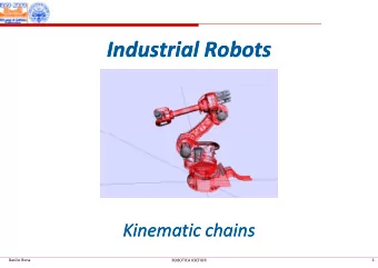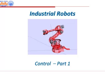
Industrial Robots Industrial Robots Control Control Part 2 Control - PowerPoint PPT Presentation
Industrial Robots Industrial Robots Control Control Part 2 Control Control Part 2 Part 2 Part 2 Introduction to centralized control Independent joint decentralized control may prove inadequate when the user requires high task
Industrial Robots Industrial Robots Control Control – Part 2 Control Control Part 2 Part 2 Part 2
Introduction to centralized control � Independent joint decentralized control may prove inadequate when � the user requires high task velocities ⇒ structured disturbance torques (Coriolis, centrifugal) greatly influence the robot behavior � motors are of direct drive type ⇒ since non gearboxes are present, their beneficial effect is absent and nonlinear effects and coupling effects become important � In these cases the disturbances torques may cause large errors on the reference trajectory tracking Basilio Bona 2 ROBOTICA 03CFIOR
Introduction to centralized control � Since in these cases it is not possible to sufficiently reduce the effects due to the disturbance torques, it is more convenient to try to cancel such torques, adopting control algorithms that use nonlinear compensation terms � We call this architecture “ centralized ” since the applied joint command torques are function also of the other joint positions and velocities. The approach is not “local” anymore, as happens in the decentralized architecture, where each joint controller uses only the local joint information (position and velocity) Basilio Bona 3 ROBOTICA 03CFIOR
Centralized control � In the centralized control architectures the robot is considered as a MIMO system, with n inputs (the joint torques) and n outputs (the joint positions ) that interact with each other ( h j i i i ) h i i h h h according to the nonlinear dynamic equations of the robot model model � The centralized control algorithms shall take into account this dynamic model, and usually they have a nonlinear form � The main centralized control architecture is called inverse inverse dynamics dynamics , since the command torques are computed from the robot dynamic equation and from the knowledge of the joint variables (positions and velocities), i.e., as a solution of an inverse dynamic problem Basilio Bona 4 ROBOTICA 03CFIOR
Inverse dynamics control Consider again the following simplified dynamic model of the robot �� + � = M q q ( ) ( ) q q h q q ( , ) ( , ) q q u c c We can compute a control command as a function of the dynamic model, where the inertia and disturbance terms are approximate where the inertia and disturbance terms are approximate � h Reference acceleration � q �� q + � r + M ROBOT ROBOT u + q q c c – a c � � � � − + u � M ( q a ) h Additional acceleration c r c command signal Basilio Bona 5 ROBOTICA 03CFIOR
Approximate linearization Hence, developing the previous equation, we have: � � �� + � = �� − + M q q ( ) h q q ( , ) M ( q a ) h r c ( ) � � − − �� = 1 �� − − 1 � − q M ( ) q M ( q a ) M ( ) q h q q ( , ) h r c ( ( ) ) � � − 1 ( ) = + M q M I E q ( ) � − = Δ � h q q ( , ) ( , ) q q h h q q ( , ) ( , ) q q � − 1 = − E q ( ) M ( ) q M I Here we try to invert the inertia matrix Here we try to invert the inertia matrix Here we try to send to zero the disturbance Here we try to send to zero the disturbance terms Basilio Bona 6 ROBOTICA 03CFIOR
Conclusions ( ) �� = �� − + η � �� q ( q a ) q q q , , , v r c r c If we can cancel this part, the system becomes linear and decoupled, but unstable Structured disturbance ( ) − η � �� = �� − − 1 Δ � q q q a E q q a M q h q q , , , ( ) ( ) ( ) ( , ) r c r c Approximation Approximation in i i in inertia model i d l Coriolis model Basilio Bona 7 ROBOTICA 03CFIOR
In general If we are able to compute the exact model of the nonlinear dynamical system, we can build the following control architecture, where a c is a suitable acceleration control signal, whose definition will allow to obtain asymptotic stability and other performances q a c u ROBOT ROBOT M q M q ( ) ( ) + + + � q � h q q ( , ) Basilio Bona 8 ROBOTICA 03CFIOR
Exact linearization and decoupling The control scheme above performs an exact system linearization The resulting system is decoupled: it consists in n double integrators; the i ‐ th component a c i of the new acceleration signal g p g c,i influences only the behavior of the i ‐ th joint component q c,i that is independent of the other joints motion q a c u q � a c q M q ( ) ROBOT ∫ ∫ + + � q � h q q ( , ) Basilio Bona 9 ROBOTICA 03CFIOR
State variable representation Basilio Bona 10 ROBOTICA 03CFIOR
Error variable representation This term is equivalent to the injection into the system of a structured nonlinear disturbance that can make it unstable in spite of the control design Basilio Bona 11 ROBOTICA 03CFIOR
Controller design Basilio Bona 12 ROBOTICA 03CFIOR
Controller design � Nonlinear Inner Loop h h ROBOT ROBOT � q q �� q q + � r + M h , M u + q q c – a c Linear Outer Loop Basilio Bona 13 ROBOTICA 03CFIOR
Inner loop – outer loop (nonlinear linearizing control) Basilio Bona 14 ROBOTICA 03CFIOR
Exact linearization Basilio Bona 15 ROBOTICA 03CFIOR
Exact linearization � h q q ( , ) ROBOT ROBOT � � q u �� q + + c M q ( ) M h , r q + – a Inner Loop c 1 1 � q q �� s s q + 1 1 r � � 1 1 – � q a q s s n n c c n n Control design Basilio Bona 16 ROBOTICA 03CFIOR
PD outer loop control design Basilio Bona 17 ROBOTICA 03CFIOR
PD outer loop control design Basilio Bona 18 ROBOTICA 03CFIOR
PD outer loop control design Inner Loop Inner Loop � h q q ( , ) ROBOT � � q u �� q + + c M q ( ) M h , r q + – a c Outer Loop � q q + + − K + r D + – q q + + − K r P – Basilio Bona 19 ROBOTICA 03CFIOR
PID outer loop control design Basilio Bona 20 ROBOTICA 03CFIOR
PID outer loop control design Inner Loop Inner Loop h � q �� q u + M r + c q ROBOT + – a c Outer Loop a PID controller for the outer loop � q + − K r + + D − − K K – + q q I r + − K s P – Basilio Bona 21 ROBOTICA 03CFIOR
PID outer loop control design Basilio Bona 22 ROBOTICA 03CFIOR
Practical aspects of exact linearization Exact linearization hypothesis implies the capacity to compute on ‐ line the model matrices � Dynamic models must be perfectly known, without errors or approximations � The model matrices must be computed online; at every sampling time (approx. 1 ms) the inverse dynamics equations must be solved Software and hardware architectures must be able to do solved. Software and hardware architectures must be able to do so � Unmodeled dynamics (e g elastic vibrations) are not taken into � Unmodeled dynamics (e.g., elastic vibrations) are not taken into account In practice it is impossible to satisfy all these assumptions at In practice it is impossible to satisfy all these assumptions at the same time Basilio Bona 23 ROBOTICA 03CFIOR
Approximate linearization � In practice one may adopt a control scheme based on the imperfect compensation of the robot inverse dynamics � There are different possibilities to do so: p 1. Only a part of the robot dynamics is computed and used in the controller (usually the dominant one and/or that is best known), leaving to the outer loop the task of guaranteeing the overall stability and the reference trajectory tracking 2. A feedforward compensation of the robot dynamics; it uses the reference values of the desired trajectory instead of the real measured joint variables and velocities to build the model measured joint variables and velocities to build the model matrices Basilio Bona 24 ROBOTICA 03CFIOR
Approximate linearization 3. Robust control techniques; these are advanced techniques that allow to overcome the effects of the approximations and other errors introduced by the real ‐ time computation of the inverse i d d b h l i i f h i dynamics 4. Adaptive control techniques; they provide an online estimation 4 Adaptive control techniques; they provide an online estimation of the true model parameters that are successively used in the controller controller � Also for the outer loop controller it is possible to adopt more complex algorithms than the simple PD controller. complex algorithms than the simple PD controller. � A PID controller will be able to cancel the steady state effects of any additive constant disturbance that the inner loop cannot y p cancel Basilio Bona 25 ROBOTICA 03CFIOR
Approximate linearization Basilio Bona 26 ROBOTICA 03CFIOR
Approximate linearization � Under the assumption that only an approximate compensation is possible, the external control law becomes: � ( ) � = + � u M q a h q q ( , ) c c Where � � M � M ; h � h represents an estimate of the true matrices. These matrices could be both the best available approximation of the true matrices, or the result of an “a ‐ priori” decision that simplifies the model i lifi h d l Basilio Bona 27 ROBOTICA 03CFIOR
Approximate linearization Inner loop Inner loop � h � q �� q u + � r + c q ROBOT M + – a c We assume to use a PD controller for the outer loop Basilio Bona 28 ROBOTICA 03CFIOR
Recommend
More recommend
Explore More Topics
Stay informed with curated content and fresh updates.
