Maximum-Likelihood Estimation The EM algorithm based on a - PDF document
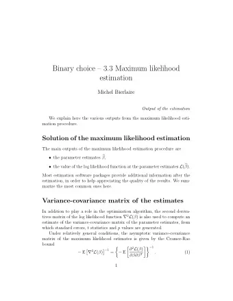
Maximum-Likelihood Estimation The EM algorithm based on a presentation by Dan Klein We have some data X and a probabilistic model P(X | ) A very general and well-studied algorithm for that data I cover only the specific case we use
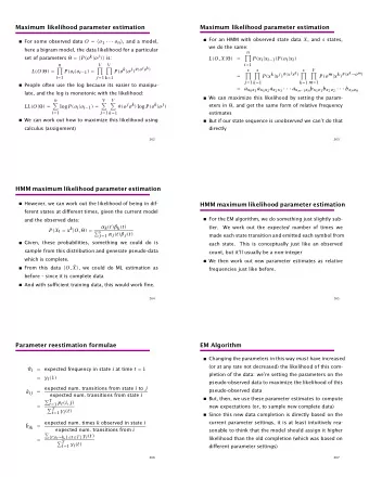
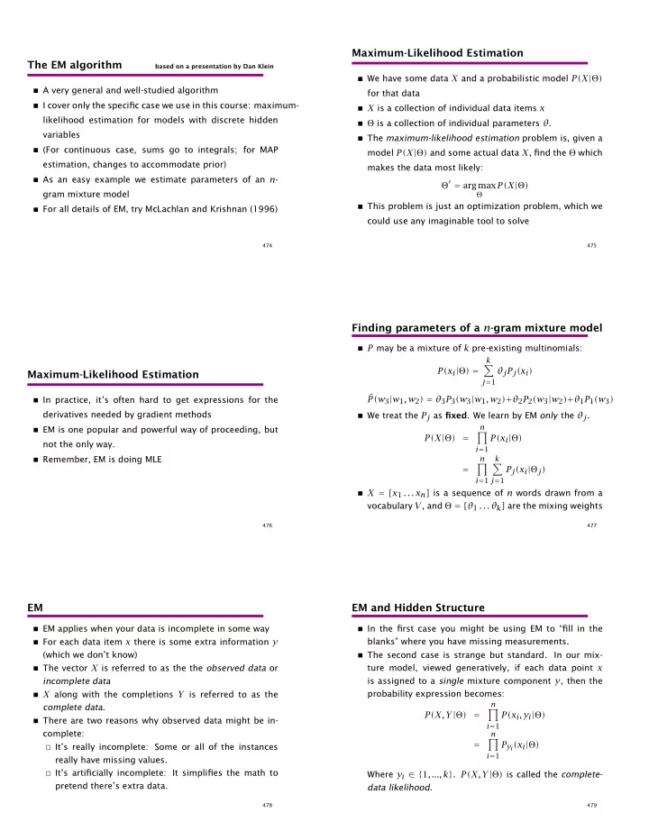
Maximum-Likelihood Estimation The EM algorithm based on a presentation by Dan Klein � We have some data X and a probabilistic model P(X | Θ ) � A very general and well-studied algorithm for that data � I cover only the specific case we use in this course: maximum- � X is a collection of individual data items x likelihood estimation for models with discrete hidden � Θ is a collection of individual parameters θ . variables � The maximum-likelihood estimation problem is, given a � (For continuous case, sums go to integrals; for MAP model P(X | Θ ) and some actual data X , find the Θ which estimation, changes to accommodate prior) makes the data most likely: � As an easy example we estimate parameters of an n - Θ ′ = arg max P(X | Θ ) gram mixture model Θ � This problem is just an optimization problem, which we � For all details of EM, try McLachlan and Krishnan (1996) could use any imaginable tool to solve 474 475 Finding parameters of a n -gram mixture model � P may be a mixture of k pre-existing multinomials: k � P(x i | Θ ) = θ j P j (x i ) Maximum-Likelihood Estimation j = 1 ˆ P(w 3 | w 1 , w 2 ) = θ 3 P 3 (w 3 | w 1 , w 2 ) + θ 2 P 2 (w 3 | w 2 ) + θ 1 P 1 (w 3 ) � In practice, it’s often hard to get expressions for the derivatives needed by gradient methods � We treat the P j as fixed . We learn by EM only the θ j . n � EM is one popular and powerful way of proceeding, but � P(X | Θ ) = P(x i | Θ ) not the only way. i = 1 � Remember, EM is doing MLE n k � � = P j (x i | Θ j ) i = 1 j = 1 � X = [x 1 . . . x n ] is a sequence of n words drawn from a vocabulary V , and Θ = [θ 1 . . . θ k ] are the mixing weights 476 477 EM EM and Hidden Structure � EM applies when your data is incomplete in some way � In the first case you might be using EM to “fill in the � For each data item x there is some extra information y blanks” where you have missing measurements. (which we don’t know) � The second case is strange but standard. In our mix- � The vector X is referred to as the the observed data or ture model, viewed generatively, if each data point x incomplete data is assigned to a single mixture component y , then the � X along with the completions Y is referred to as the probability expression becomes: n complete data . � P(X, Y | Θ ) = P(x i , y i | Θ ) � There are two reasons why observed data might be in- i = 1 complete: n � = P y i (x i | Θ ) � It’s really incomplete: Some or all of the instances i = 1 really have missing values. � It’s artificially incomplete: It simplifies the math to Where y i ∈ { 1 , ..., k } . P(X, Y | Θ ) is called the complete- pretend there’s extra data. data likelihood . 478 479
EM and Hidden Structure EM and Hidden Structure � Note: � Looking at completions is useful because finding � the sum over components is gone, since y i tells us Θ = arg max P(X | Θ ) which single component x i came from. We just don’t Θ is hard (it’s our original problem – maximizing products know what the y i are. � our model for the observed data X involved the “un- of sums is hard) observed” structures – the component indexes – all � On the other hand, finding along. When we wanted the observed-data likelihood Θ = arg max P(X, Y | Θ ) we summed out over indexes. Θ would be easy – if we knew Y . � there are two likelihoods floating around: the observed- � The general idea behind EM is to alternate between max- data likelihood P(X | Θ ) and the complete-data like- imizing Θ with Y fixed and “filling in” the completions Y lihood P(X, Y | Θ ) . EM is a method for maximizing based on our best guesses given Θ . P(X | Θ ) . 480 481 The EM algorithm The EM algorithm � In the E-step we calculate the likelihood of the various completions with our fixed Θ ′ . � The actual algorithm is as follows: Initialize Start with a guess at Θ – it may be a very bad � In the M-stem we maximize the expected log-likelihood guess of the complete data. That’s not the same thing as the Until tired likelihood of the observed data, but it’s close E-Step Given a current, fixed Θ ′ , calculate comple- � The hope is that even relatively poor guesses at Θ , when tions: P(Y | X, Θ ′ ) constrained by the actual data X , will still produce de- M-Step Given fixed completions P(Y | X, Θ ′ ) , maximize cent completions Y P(Y | X, Θ ′ ) log P(X, Y | Θ ) with respect to Θ . � � Note that “the complete data” changes with each itera- tion 482 483 EM made easy EM made easy � Want: Θ which maximizes the data likelihood � Want: a product of products L( Θ ) = P(X | Θ ) � Arithmetic-mean-geometric-mean (AMGM) inequality says � = Y P(X, Y | Θ ) that, if � i w i = 1 , � The Y ranges over all possible completions of X . Since z w i � � ≤ w i z i i X and Y are vectors of independent data items, i � � L( Θ ) = P(x, y | Θ ) � In other words, arithmetic means are larger than geo- x y metric means (for 1 and 9, arithmetic mean is 5, geo- � We don’t want a product of sums. It’d be easy to maxi- metric mean is 3) mize if we had a product of products. � This equality is promising, since we have a sum and � Each x is a data item, which is broken into a sum of want a product sub-possibilties, one for each completion y . We want to make each completion be like a mini data item, all � We can use P(x, y | Θ ) as the z i , but where do the w i multiplied together with other data items. come from? 484 485
EM made easy EM made easy � Then, we would have � The answer is to bring our previous guess at Θ into the � � y P(x, y | Θ ) x R( Θ | Θ ′ ) = picture. x P(x | Θ ′ ) � � Let’s assume our old guess was Θ ′ . Then the old likeli- � y P(x, y | Θ ) � = P(x | Θ ′ ) hood was x P(x, y | Θ ) L( Θ ′ ) = P(x | Θ ′ ) � � � = P(x | Θ ′ ) x x y P(y | x, Θ ′ ) � This is just a constant . So rather than trying to make P(x, y | Θ ) � � = P(x | Θ ′ ) P(y | x, Θ ′ ) L( Θ ) large, we could try to make the relative change in x y P(y | x, Θ ′ ) P(x, y | Θ ) likelihood � � = P(x, y | Θ ′ ) R( Θ | Θ ′ ) = L( Θ ) x y L( Θ ′ ) � Now that’s promising: we’ve got a sum of relative likeli- large. hoods P(x, y | Θ )/P(x, y | Θ ′ ) weighted by P(y | x, Θ ′ ) . 486 487 EM made easy EM made easy � We can use our identity to turn the sum into a product: P(y | x, Θ ′ ) P(x, y | Θ ) � We started trying to maximize the likelihood L( Θ ) and R( Θ | Θ ′ ) = � � P(x, y | Θ ′ ) x y saw that we could just as well maximize the relative � P(y | x, Θ ′ ) � likelihood R( Θ | Θ ′ ) = L( Θ )/L( Θ ′ ) . But R( Θ | Θ ′ ) was still P(x, y | Θ ) � � ≥ P(x, y | Θ ′ ) a product of sums, so we used the AMGM inequality and x y � Θ , which we’re maximizing, is a variable, but Θ ′ is just found a quantity Q( Θ | Θ ′ ) which was (proportional to) a a constant. So we can just maximize lower bound on R . That’s useful because Q is something P(x, y | Θ ) P(y | x, Θ ′ ) that is easy to maximize, if we know P(y | x, Θ ′ ) . Q( Θ | Θ ′ ) = � � x y 488 489 The EM Algorithm � The first step is called the E-Step because we calculate The EM Algorithm the expected likelihoods of the completions. � So here’s EM, again: � The second step is called the M-Step because, using � Start with an initial guess Θ ′ . those completion likelihoods, we maximize Q , which hopefully increases R and hence our original goal L � Iteratively do E-Step Calculate P(y | x, Θ ′ ) � The expectations give the shape of a simple Q function M-Step Maximize Q( Θ | Θ ′ ) to find a new Θ ′ for that iteration, which is a lower bound on L (because of AMGM). At each M-Step, we maximize that lower bound � In practice, maximizing Q is just setting parameters as � This procedure increases L at every iteration until Θ ′ relative frequencies in the complete data – these are the reaches a local extreme of L . maximum likelihood estimates of Θ � This is because successive Q functions are better ap- proximations, until you get to a (local) maxima 490 491
Recommend
More recommend
Explore More Topics
Stay informed with curated content and fresh updates.
