Maximum likelihood estimation of factor models on data sets with - PowerPoint PPT Presentation

Maximum likelihood estimation of factor models on data sets with arbitrary pattern of missing data. Marta Ba´ nbura Michele Modugno European Central Bank 6th Eurostat Colloquium, 29 September 2010

Framework Dynamic factor model y t Λ f t + ε t = f t A 1 f t − 1 + · · · + A p f t − p + u t = • State space form. • Factors are unobservable. • Factors follow a VAR dynamic.

Framework Dynamic factor model y t Λ f t + ε t = f t A 1 f t − 1 + · · · + A p f t − p + u t = • State space form. • Factors are unobservable. • Factors follow a VAR dynamic. • y t can follow an arbitrary pattern of missing data .

Arbitrary pattern of missing data -2.09 0.70 -11.59 NaN NaN NaN NaN NaN NaN -2.17 2.19 -12.04 NaN NaN NaN NaN NaN NaN -1.79 -3.19 -9.92 NaN NaN NaN 0.10 0.23 0.08 -1.04 -9.75 -5.78 0.89 NaN NaN NaN NaN NaN -0.28 -7.79 -1.54 -0.70 NaN NaN NaN NaN NaN 0.10 -0.05 0.57 0.47 0.54 -0.96 -0.10 0.32 -0.08 NaN 4.22 -0.93 1.45 -0.15 0.19 NaN NaN NaN -0.43 0.43 -2.42 2.45 -0.22 0.80 NaN NaN NaN 0.06 -13.71 0.33 3.13 0.57 0.09 1.20 0.57 0.96 0.09 NaN 0.51 3.05 0.32 0.04 NaN NaN NaN 0.12 -13.15 0.64 1.70 -0.07 -1.47 NaN NaN NaN -0.53 -8.77 -2.92 1.03 0.28 -1.10 0.30 0.87 0.24 -1.27 -8.21 -7.04 0.38 0.25 -0.75 NaN NaN NaN -1.53 -7.94 -8.52 1.36 0.29 -0.74 NaN NaN NaN -1.10 -9.46 -6.12 2.13 -0.06 -1.23 0.50 0.70 0.4 -0.69 2.48 -3.82 NaN -0.24 4.70 NaN NaN NaN -0.93 NaN -5.17 NaN NaN NaN NaN NaN NaN NaN NaN NaN NaN NaN NaN NaN NaN NaN

Estimation of dynamic factor model For small scale models: Maximum likelihood • Use of optimisation methods: • In the time domain (Engle and Watson, 1981, Quah and Sargent, 1992) • In the frequency domain domain (Geweke, 1977; Sargent and Sims, 1977) • EM algorithm (Watson and Engle, 1983, Shumway and Stoffer, 1982) With missing data: Shumway and Stoffer, 1982 only if the the loading matrix is known!

Estimation of dynamic factor model For large scale models: • Principal components (Connor and Korajczyk (1986,1988),Forni and Reichlin (1996,1998), Forni, Hallin, Lippi and Reichlin (2000), Stock and Watson (2002)) With missing data: Giannone, Reichlin and Small(2008) only at the end of the sample! • Maximum likelihood with EM algorithm Doz, Giannone, and Reichlin (2006): Likelihood for a misspecified model: no serial and cross-correlation of the idiosyncratic components if N , T → + ∞ , no problem!

Contributions of this paper Generalize Doz, Giannone, and Reichlin (2006) in order to: • adapt EM algorithm to deal with a general pattern of missing data • introduce restrictions on the parameters: group specific factors • model dynamics of idiosyncratic component Moreover: • Monte Carlo evaluation • News concept: helps to understand the sources of forecast revisions in case of multiple data releases • Application to the euro area data: real-time forecasting and backdating of GDP

EM, how does it work Solution to problems in which latent or missing data yield the likelihood intractable. Write the likelihood as if all the data were observed: in terms of both observables and factors . Iterate: • E-step : replace the sufficient statistics by their expectations (given the parameters from previous iteration) • M-step : maximise the “expected likelihood”

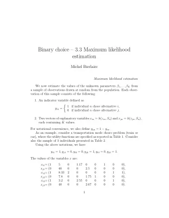
EM, dynamic factor model y t Λ f t + ξ t , ξ t ∼ N ( 0 , R ) = f t Af t − 1 + u t , u t ∼ N ( 0 , Q ) = f t observed and y t available : � T � � T � − 1 � � y t f ′ f t f ′ � Λ = t t t = 1 t = 1 � T � � � � � T T � � � � ′ � � � 1 1 R � diag y t − ˆ Λ f t y t − ˆ Λ f t = diag y t y ′ t − ˆ f t y ′ = Λ t T T t = 1 t = 1 t = 1

EM, dynamic factor model f t unobserved and y t available (EM, Ω T = Data): � T � � T � − 1 � � � � � � Λ( r + 1 ) y t f ′ f t f ′ E θ ( r ) E θ ( r ) � = t | Ω T t | Ω T t = 1 t = 1 � � T � � T � � � � � � 1 R ( r + 1 ) diag E θ ( r ) y t y ′ Λ( r + 1 ) E θ ( r ) f t y ′ � − � = t | Ω T t | Ω T T t = 1 t = 1 Analogously for A and Q in the state equation. Expectations of the sufficient statistics without missing data (Watson and Engle, 1983) � � � � � � • E θ ( r ) y t f ′ = y t E θ ( r ) f ′ or E θ ( r ) y t y ′ = y t y ′ t | Ω T t | Ω T t | Ω T t � � � � • E θ ( r ) f ′ or E θ ( r ) f t − 1 f ′ t | Ω T t − 1 | Ω T from the Kalman smoother

EM for the factor model, y t contains missing values y t with missing data ⇒ we cannot longer use Watson and Engle, 1983 Instead � T � − 1 � T � � � �� � � � � � vec Λ( r + 1 ) E θ ( r ) f t f ′ ⊗ W t vec W t y t E θ ( r ) f ′ = t | Ω T t | Ω T t = 1 t = 1 � T � � � �� 1 R ( r + 1 ) = diag W t y t y ′ t W ′ t − W t y t E θ ( r ) f ′ Λ( r + 1 ) ′ W t + � t | Ω T T t = 1 � � − W t � Λ( r + 1 ) E θ ( r ) f t | Ω T y ′ t W ′ t + W t � Λ( r + 1 ) �� � �� E θ ( r ) f t f ′ Λ( r + 1 ) ′ W t + ( I − W t ) � R ( r )( I − W t ) t | Ω T

Application: Daily Inflation Tracking Proposes a framework to nowcast and forecast the euro area HICP inflation exploiting weekly and daily data. HICP data are published 15 days after the end of the reference month. Only for Total HICP there is a flash estimate for the current month, released at the end of the month. However, till the end of the month, weekly and daily data are available. We want to exploit this information in order to know where inflation is, before the flash estimate is published.

Data We focus on two groups of series. The first is: The Weekly Commission Oil Bulletin Price Statistics (WOB) . Member states initiated a survey to gather data on petroleum prices. Every Monday they communicate to the European Commission consumer prices of petroleum products net of duties and taxes and inclusive all duties and taxes in force. This data are average through the period. Focus on the consumer prices . In comparison to raw oil prices they account for distribution and retail margins . (released 2 or 3 days after the reference period)

Data The second group of data are. World Market Prices of Raw Materials (RMP) . Weighted according to commodity imports of Euro area countries in 1999-2001, excluding EU-intra trade. Published at mid of following week. Raw Material Prices capture some of the global price dynamics as well as prices at the early part of the pricing chain. (released 2 or 3 days after the reference period)

Why RMP and WOB? Coincident! 1/4/2005 -3.5 -2.5 -1.5 -0.5 0.5 1.5 2.5 1/7/2005 1/10/2005 1/1/2006 1/4/2006 1/7/2006 1/10/2006 1/1/2007 1/4/2007 1/7/2007 1/10/2007 1/1/2008 1/4/2008 1/7/2008 1/10/2008 1/1/2009 1/4/2009 1/7/2009 1/10/2009 total RMP Gas oil Euro Super 95 Diesel overall HICP

Why RMP and WOB? More timely! March 2010 HICP Flash Releases Estimate Feb 10 Mar 10 ↓ ↓ > .. .. 15 16 .. 22 23 26 .. 29 30 1 2 3 4 5 8 9 10 11 12 17 18 19 24 25 31 ↑ ↑ ↑ ↑ ↑ ↑ ↑ ↑ ↑ ↑ RMP RMP RMP RMP RMP 22-26 Feb 1-5 Mar 8-12 Mar 15-19 Mar 22-26 Mar WOB WOB WOB WOB WOB 23 Feb - 1 Mar 2-8 Mar 9-15 Mar 16-22 Mar 23-29 Mar

Literature Review The use of higher frequency indicators in order to Nowcast/Forecast lower frequency indicators started with monthly data for GDP , among others Giannone, Reichlin and Small (2008) for the U.S. and Banbura and Runstler (2007) for the Euro Area show that using monthly indicators is crucial in order to Nowcast accurately GDP . For inflation Monteforte and Moretti (2010) extract from daily financial series some factors that are then plugged in an equation (predetermination) for forecasting inflation . These daily factors are then averaged using a MIDAS regression.

Literature Review The use of higher frequency indicators in order to Nowcast/Forecast lower frequency indicators started with monthly data for GDP , among others Giannone, Reichlin and Small (2008) for the U.S. and Banbura and Runstler (2007) for the Euro Area show that using monthly indicators is crucial in order to Nowcast accurately GDP . For inflation Monteforte and Moretti (2010) extract from daily financial series some factors that are then plugged in an equation (predetermination) for forecasting inflation . These daily factors are then averaged using a MIDAS regression. ⇒ do not use the full co-movement to extract the signal

Literature Review The use of higher frequency indicators in order to Nowcast/Forecast lower frequency indicators started with monthly data for GDP , among others Giannone, Reichlin and Small (2008) for the U.S. and Banbura and Runstler (2007) for the Euro Area show that using monthly indicators is crucial in order to Nowcast accurately GDP . For inflation Monteforte and Moretti (2010) extract from daily financial series some factors that are then plugged in an equation (predetermination) for forecasting inflation . These daily factors are then averaged using a MIDAS regression. ⇒ do not use the full co-movement to extract the signal ⇒ daily variables are predetermined: no unique framework for forecasting all the variables, no News