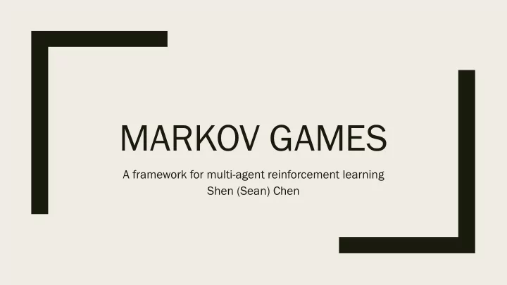
MARKOV GAMES A framework for multi-agent reinforcement learning - PowerPoint PPT Presentation
MARKOV GAMES A framework for multi-agent reinforcement learning Shen (Sean) Chen Review on MDPs An MDP is defined by a set of states, S, and actions, A. Transition function, T: S A PD(S), where PD(S) represents discrete prob
MARKOV GAMES A framework for multi-agent reinforcement learning Shen (Sean) Chen
Review on MDP’s ■ An MDP is defined by a set of states, S, and actions, A. Transition function, T: S × A → PD(S), where PD(S) represents discrete prob ■ distribution over the set S. Reward function, R: S × A → R, which specifies the agent’s task ■ ■ Objective: find a policy mapping its interaction history to a current choice of action ( 𝛿 % 𝑠 +,% so as to maximize the expected sum of discounted reward 𝐹 ∑ %&'
Markov Games ■ A Markov game is defined by a set of states S, and a collection of action sets, 𝐵 . , 𝐵 0 , … , 𝐵 2 , one for each agent in the environment. ■ State transitions are controlled by the current state and one action from each agent: T: S × 𝐵 . × 𝐵 0 × ⋯× 𝐵 2 → PD(S). Reward function associated to each agent i: 𝑆 5 : S × 𝐵 . × 𝐵 0 × ⋯× 𝐵 2 → R ■ ( 𝛿 % 𝑠 5, +,% , where 𝑠 5, +,% is the reward Objective: find a policy that maximizes 𝐹 ∑ %&' ■ received j steps into the future by agent i
MDP’s VS Markov Games ■ MDP: – Assumes stationarity in the environment – Learns deterministic policies, hence agents not Adaptive ■ Markov Games: – An extension of game theory to MDP-like environments – Include multiple adaptive agents with interactive or competing goals – Minimax strategy allows the agent to converge to a fixed strategy that is guaranteed to be ‘safe’ in that it does not as well as possible against the worst possible opponent
Optimal Policy – Matrix Games ■ Every two-player, simultaneous-move, zero-sum game has a Nash equilibrium ■ Suppose we have two agents: A and O ∗ , 𝜌 : ∗ , where V is from the perspective of A Value V = 𝐹 π 7 ■ ∗ , 𝜌 : ≥ 𝑊 𝐹 π 7 ■ ∗ ≤ 𝑊 𝐹 𝜌 7 , 𝜌 : ■
Optimal Policy – Matrix Games ■ The agent’s policy is a probability distribution over actions ■ The optimal agent’s minimum expected reward should be as large as possible ■ Imagine a policy that is guaranteed an expected score of V no matter what action the opponent chooses ■ For pi to be optimal, we must identify the largest V for which there is some value of pi that makes the constraints hold, using linear programming :∈I ∑ 7∈F 𝑆 :,7 𝜌 7 , ■ Objective: 𝑊 = B∈DE F min max
Optimal Policy – MDP’s ■ Method: Value Iteration Quality of a state-action pair: the total expected discounted reward attained by the non-stationary ■ Qu policy that takes action a at state s 𝑅 𝑡, 𝑏 = 𝑆 𝑡, 𝑏 + 𝛿 ∑ N O ∈P 𝑈 𝑡, 𝑏, 𝑡 R 𝑊 𝑡 R Immediate reward plus discounted value of all succeeding states weighted by likelihood Value of a state: the total expected discounted reward attained by policy starting from state s ■ Va 7 O ∈ F 𝑅 𝑡, 𝑏 R 𝑊 𝑡 = max Quality of the best action for that state; ■ Knowing Q is enough to specify an optimal policy, because action can be chosen with the the highest Q-value in each state
Optimal Policy – Markov Games ■ Redefine V(s): expected reward for the optima policy starting from state s 𝑊 = B∈DE F min max :∈I S Q s, a, o 𝜌 7 , 7∈F For games with alternating t turns , i.e. optimal de deterministic policy, V(s) need not be computed by LP 𝑊 = max 7∈F min :∈I 𝑅(𝑡, 𝑏, 𝑝) ■ Q(s, a, o): expected reward for taking action a when the opponent chooses o from state s and continuing optimally thereafter 𝑈 𝑡, 𝑏, 𝑝, 𝑡 R 𝑊 𝑡 R 𝑅 𝑡, 𝑏, 𝑝 = 𝑆 𝑡, 𝑏, 𝑝 + 𝛿 S N O ∈P ■ Analogous value iteration algorithm can be shown to converge to the correct values
Optimal Policy – Learning Process ■ Minimax-Q: Alternative approach to tradition value iteration method: 𝑅 𝑡, 𝑏 ≔ 𝑠 + 𝛿𝑊 𝑡 R – Performing the updates asynchronously without the use of the transition T – The probability of the update is precisely T – The rule converges to the correct value of Q & V if ■ Every action is tried in every state infinitely often ■ The new estimates are blended with previous ones using a slow e enough exponentially w weighted a average
Experiments ■ A minmax-Q learning algorithm using a simple two-player zero-sum markov game modelled after the game of soccer ■ Consider a well-studied specialization in which there are only two agents and they have diametrically opposed goals.
Experiments – Soccer Game ■ Actions: N, S, E, W, stand ■ Two moves are executed in random order ■ Circle represents the ball ■ Goals: left A, right B ■ Possession of the ball randomly initialized when game is reset ■ Discount factor 0.9 ■ To do better than breaking even against an unknown defender, an offensive agent must use a probabilistic policy
Experiments – Training and Testing Four different Policies learnt: Using minmax-Q: explor = 0.2, decay = 10 (]^_ '.'.)/.' b = 0.9999954 ■ MR: minimax-Q trained against uniformly random ■ MM: minimax-Q trained against minimax (separate Q & V-tables) Using Q-learning: ‘max’ operator used in place of minimax; Q-table not tracking opponent’s actions ■ QR: Q trained against uniformly random ■ QQ: Q trained against Q (separate Q & V-tables)
Experiments – Training and Testing Three ways of valuation on the resulting policies ■ First, each policy was run head-to-head with a random policy for 100,000 steps – To emulate the discount factor, every step had a 0.1 probability of being declared a draw – Wins and losses against the random opponent were tabulated ■ Second, head-to-head competition with a hand-built policy. – Hand-built policy was deterministic and had simple rules for scoring and blocking ■ Third, use –learning to train a ‘challenger’ opponent for each of MR, MM, QR, QQ. – The training policy followed that of QR, where the ‘champion’ policy was held while the challenger was trained against it. – The resulting policies were evaluated against their respective champions
Experiments – Results
Discussion and Questions ■ Why is it that in games such as checkers, backgammon and Go, "the minimax operator (in minimax Q) can be implemented extremely efficiently." Does the optimal strategy/policy always need to be mixed? Can it be pure, e.g. 𝜌 = ■ (0, 1,0) ? How would you design a markov game in which only pure strategies would be sufficient? ■ What if we have two sets of rewards for the agents, rather than a zero-sum setting? ■ Will mini-max/max-min strategy work for n-player game?
Recommend
More recommend
Explore More Topics
Stay informed with curated content and fresh updates.
