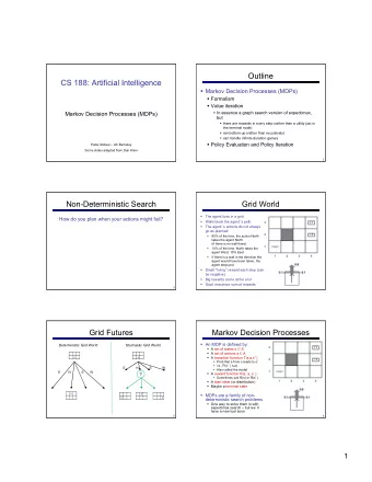
Markov Decision Processes (MDPs) Machine Learning 10701/15781 - PowerPoint PPT Presentation

Reading: Kaelbling et al. 1996 (see class website) Markov Decision Processes (MDPs) Machine Learning – 10701/15781 Carlos Guestrin Carnegie Mellon University May 1 st , 2006 1

Announcements � Project: � Poster session: Friday May 5 th 2-5pm, NSH Atrium � please arrive a little early to set up � FCEs!!!! � Please, please, please, please, please, please give us your feedback, it helps us improve the class! ☺ � http://www.cmu.edu/fce 2

Discount Factors People in economics and probabilistic decision-making do this all the time. The “Discounted sum of future rewards” using discount factor γ ” is (reward now) + γ (reward in 1 time step) + γ 2 (reward in 2 time steps) + γ 3 (reward in 3 time steps) + : : (infinite sum) 3

t n u o c s D i e m The Academic Life u s 9 s . 0 A γ = r o t c a F 0.6 0.6 0.2 0.2 0.7 B. A. T. Assoc. Assistant Tenured Prof Prof Prof 60 20 400 0.2 S. 0.2 0.3 D. On the Dead Street 0 10 Define: 0.7 0.3 V A = Expected discounted future rewards starting in state A V B = Expected discounted future rewards starting in state B V T = “ “ “ “ “ “ “ T V S = “ “ “ “ “ “ “ S V D = “ “ “ “ “ “ “ D How do we compute V A , V B , V T , V S , V D ? 4

Computing the Future Rewards of an Academic 0.6 0.6 0.7 0.2 0.2 B. A. T. Assoc. Assistant Tenured Prof Prof Prof 60 20 400 S. 0.2 0.2 0.3 D. On the Dead Street 0 10 0.7 0.3 Assume Discount Factor γ = 0.9 5

Joint Decision Space Markov Decision Process (MDP) Representation: � State space: � Joint state x of entire system � Action space: � Joint action a = {a 1 ,…, a n } for all agents � Reward function: � Total reward R( x , a ) � sometimes reward can depend on action � Transition model: � Dynamics of the entire system P( x ’| x , a ) 6

Policy At state x , Policy: π ( x ) = a action a for all agents x 0 π ( x 0 ) = both peasants get wood x 1 π ( x 1 ) = one peasant builds barrack, other gets gold x 2 π ( x 2 ) = peasants get gold, footmen attack 7

Value of Policy Expected long- Value: V π ( x ) term reward starting from x V π ( x 0 ) = E π [R( x 0 ) + γ R( x 1 ) + γ 2 R( x 2 ) + Start γ 3 R( x 3 ) + γ 4 R( x 4 ) + L ] from x 0 π (x 0 ) x 0 Future rewards x 1 π (x 1 ) discounted by γ ∈ [0,1) R(x 0 ) x 2 π (x 2 ) R(x 1 ) π ( x 1 ’ ) x 3 π (x 3 ) x 1 ’ R(x 2 ) x 4 R( x 1 ’ ) π ( x 1 ’’ ) R(x 3 ) x 1 ’’ R(x 4 ) 8 R( x 1 ’’ )

Computing the value of a policy V π ( x 0 ) = E π [R( x 0 ) + γ R( x 1 ) + γ 2 R( x 2 ) + γ 3 R( x 3 ) + γ 4 R( x 4 ) + L ] � Discounted value of a state: � value of starting from x 0 and continuing with policy π from then on � A recursion! 9

Computing the value of a policy 1 – the matrix inversion approach � Solve by simple matrix inversion: 10

Computing the value of a policy 2 – iteratively � If you have 1000,000 states, inverting a 1000,000x1000,000 matrix is hard! � Can solve using a simple convergent iterative approach: (a.k.a. dynamic programming) � Start with some guess V 0 � Iteratively say: � V t+1 = R + γ P π V t � Stop when ||V t+1 -V t || ∞ · ε � means that ||V π -V t+1 || ∞ · ε /(1- γ ) 11

But we want to learn a Policy � So far, told you how good a At state x , action Policy: π ( x ) = a a for all agents policy is… � But how can we choose the x 0 π ( x 0 ) = both peasants get wood best policy??? x 1 π ( x 1 ) = one peasant builds barrack, other gets gold � Suppose there was only one x 2 π ( x 2 ) = peasants get gold, time step: footmen attack � world is about to end!!! � select action that maximizes reward! 12

Another recursion! � Two time steps: address tradeoff � good reward now � better reward in the future 13

Unrolling the recursion � Choose actions that lead to best value in the long run � Optimal value policy achieves optimal value V * 14

Bellman equation � Evaluating policy π : � Computing the optimal value V * - Bellman equation ∑ ∗ ∗ = + γ ( ) max ( , ) ( ' | , ) ( ' ) x x a x x a x V R P V a ' x 15

Optimal Long-term Plan Optimal value Optimal Policy: π * ( x ) function V * ( x ) ∑ ∗ ∗ = + γ ( , ) ( , ) ( ' | , ) ( ' ) x a x a x x a x Q R P V ' x Optimal policy: ∗ ∗ π = ( x ) arg max ( x , a ) Q a 16

Interesting fact – Unique value ∑ ∗ ∗ = + γ ( ) max ( , ) ( ' | , ) ( ' ) x x a x x a x V R P V a ' x � Slightly surprising fact : There is only one V * that solves Bellman equation! � there may be many optimal policies that achieve V * � Surprising fact : optimal policies are good everywhere!!! 17

Solving an MDP Solve Optimal Optimal Bellman policy π * ( x ) value V * ( x ) equation ∑ ∗ ∗ = + γ ( ) max ( , ) ( ' | , ) ( ' ) x x a x x a x V R P V a ' x Bellman equation is non-linear!!! Many algorithms solve the Bellman equations: � Policy iteration [Howard ‘60, Bellman ‘57] � Value iteration [Bellman ‘57] � Linear programming [Manne ‘60] � … 18

Value iteration (a.k.a. dynamic programming) – the simplest of all ∑ ∗ ∗ = + γ ( ) max ( , ) ( ' | , ) ( ' ) x x a x x a x V R P V a ' x � Start with some guess V 0 � Iteratively say: ∑ = + γ ( ) max ( , ) ( ' | , ) ( ' ) x x a x x a x � V R P V + 1 t t a ' x � Stop when ||V t+1 -V t || ∞ · ε � means that ||V ∗ -V t+1 || ∞ · ε /(1- γ ) 19

A simple example γ = 0.9 1 S You run a 1 startup Poor & Poor & 1/2 A company. Unknown Famous A 1/2 +0 +0 In every state you S 1/2 must 1/2 1 choose 1/2 1/2 1/2 between A S Saving A 1/2 money or Rich & Rich & Advertising. Famous 1/2 S Unknown +10 1/2 +10 20

Let’s compute V t (x) for our example γ = 0.9 1 S t V t (PU) V t (PF) V t (RU) V t (RF) 1 Poor & Poor & 1/2 A Unknown Famous A 1/2 +0 +0 1 S 1/2 1/2 1 1/2 1/2 2 1/2 A S A 1/2 3 Rich & Rich & Famous S 1/2 Unknown +10 4 1/2 +10 5 6 ∑ = + γ ( ) max ( , ) ( ' | , ) ( ' ) x x a x x a x V R P V + 1 t t a ' x 21

Let’s compute V t (x) for our example γ = 0.9 1 S t V t (PU) V t (PF) V t (RU) V t (RF) 1 Poor & Poor & 1/2 A Unknown Famous A 1/2 +0 +0 1 0 0 10 10 S 1/2 1/2 1 1/2 1/2 2 0 4.5 14.5 19 1/2 A S A 1/2 3 2.03 6.53 25.08 18.55 Rich & Rich & Famous S 1/2 Unknown +10 4 3.852 12.20 29.63 19.26 1/2 +10 5 7.22 15.07 32.00 20.40 6 10.03 17.65 33.58 22.43 ∑ = + γ ( ) max ( , ) ( ' | , ) ( ' ) x x a x x a x V R P V + 1 t t a ' x 22

Policy iteration – Another approach for computing π * � Start with some guess for a policy π 0 � Iteratively say: ∑ = = π + γ = π ( ) ( , ( )) ( ' | , ( )) ( ' ) V x R x a x P x x a x V x � evaluate policy: t t t t x ' ∑ π = + γ ( ) max ( , ) ( ' | , ) ( ' ) � improve policy: x R x a P x x a V x + 1 t t a x ' � Stop when � policy stops changing � usually happens in about 10 iterations � or ||V t+1 -V t || ∞ · ε � means that ||V ∗ -V t+1 || ∞ · ε /(1- γ ) 23

Policy Iteration & Value Iteration: Which is best ??? It depends. Lots of actions? Choose Policy Iteration Already got a fair policy? Policy Iteration Few actions, acyclic? Value Iteration Best of Both Worlds: Modified Policy Iteration [Puterman] …a simple mix of value iteration and policy iteration 3 rd Approach Linear Programming 24

LP Solution to MDP [Manne ‘60] Value computed by linear programming: ∑ minimize : ( x ) V (x ) V x ∑ ⎧ ≥ + γ ( x ) V V (x ) ( , ) ( ' | , ) ( ' ) x a x x a x R P V ⎨ subject to : ∀ a ' ∀ x ⎩ , x , x a � One variable V ( x ) for each state � One constraint for each state x and action a � Polynomial time solution 25

What you need to know � What’s a Markov decision process � state, actions, transitions, rewards � a policy � value function for a policy � computing V π � Optimal value function and optimal policy � Bellman equation � Solving Bellman equation � with value iteration, policy iteration and linear programming 26

Acknowledgment � This lecture contains some material from Andrew Moore’s excellent collection of ML tutorials: � http://www.cs.cmu.edu/~awm/tutorials 27

Reading: Kaelbling et al. 1996 (see class website) Reinforcement Learning Machine Learning – 10701/15781 Carlos Guestrin Carnegie Mellon University May 1 st , 2006 28

The Reinforcement Learning task World : You are in state 34. Your immediate reward is 3. You have possible 3 actions. Robot : I’ll take action 2. World : You are in state 77. Your immediate reward is -7. You have possible 2 actions. Robot : I’ll take action 1. World : You’re in state 34 (again). Your immediate reward is 3. You have possible 3 actions. 29