10/12/2012 Logistics PS 2 due Tuesday Thursday 10/18 PS 3 due - PDF document
10/12/2012 Logistics PS 2 due Tuesday Thursday 10/18 PS 3 due Thursday 10/25 CSE 473 Markov Decision Processes Dan Weld Many slides from Chris Bishop, Mausam, Dan Klein, Stuart Russell, Andrew Moore & Luke Zettlemoyer MDPs Planning
10/12/2012 Logistics PS 2 due Tuesday Thursday 10/18 PS 3 due Thursday 10/25 CSE 473 Markov Decision Processes Dan Weld Many slides from Chris Bishop, Mausam, Dan Klein, Stuart Russell, Andrew Moore & Luke Zettlemoyer MDPs Planning Agent Static vs. Dynamic Markov Decision Processes • Planning Under Uncertainty Environment Fully • Mathematical Framework vs. • Bellman Equations Partially Deterministic ete st c Observable Ob bl • Value Iteration vs. What action Stochastic • Real ‐ Time Dynamic Programming next? Andrey Markov • Policy Iteration (1856 ‐ 1922) Perfect Instantaneous vs. vs. • Reinforcement Learning Durative Noisy Percepts Actions Objective of an MDP Review: Expectimax • Find a policy : � → � What if we don’t know what the result of an action will be? E.g., • In solitaire, next card is unknown • which optimizes max • In pacman, the ghosts act randomly • minimizes expected cost to reach a discounted Can do expectimax search goal or Max nodes as in minimax search Max nodes as in minimax search chance chance undiscount. • maximizes expected reward Chance nodes, like min nodes, except the outcome is uncertain ‐ take • maximizes expected (reward ‐ cost) average (expectation) of children Calculate expected utilities 10 4 5 7 • given a ____ horizon • finite Today, we formalize as an Markov Decision Process • infinite Handle intermediate rewards & infinite plans More efficient processing • indefinite 1
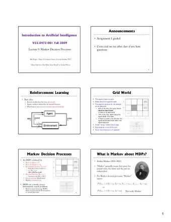
10/12/2012 Grid World Markov Decision Processes An MDP is defined by: Walls block the agent’s path • A set of states s S Agent’s actions may go astray: • A set of actions a A 80% of the time, North action • A transition function T(s,a,s’) • Prob that a from s leads to s’ takes the agent North • i.e., P(s’ | s,a) (assuming no wall) • Also called “the model” 10% ‐ actually go West • A reward function R(s, a, s’) • Sometimes just R(s) or R(s’) 10% ‐ actually go East • A start state (or distribution) If there is a wall in the chosen • Maybe a terminal state direction, the agent stays put • MDPs: non ‐ deterministic search Small “living” reward each step Reinforcement learning: MDPs where we don’t Big rewards come at the end know the transition or reward functions Goal: maximize sum of rewards What is Markov about MDPs? Solving MDPs In deterministic single-agent search problems, want an optimal Andrey Markov (1856 ‐ 1922) plan, or sequence of actions, from start to a goal “Markov” generally means that In an MDP, we want an optimal policy *: S → A • A policy gives an action for each state • conditioned on the present state, • the future is independent of the past p p • An optimal policy maximizes expected utility if followed An optimal policy maximizes expected utility if followed • Defines a reflex agent For Markov decision processes, “Markov” means: Optimal policy when R(s, a, s’) = ‐ 0.03 for all non ‐ terminals s Example Optimal Policies Example Optimal Policies R(s) = ‐ 0.01 R(s) = ‐ 0.03 R(s) = ‐ 0.01 R(s) = ‐ 0.03 R(s) = ‐ 0.4 R(s) = ‐ 0.4 R(s) = ‐ 2.0 R(s) = ‐ 2.0 2
10/12/2012 Example Optimal Policies Example Optimal Policies R(s) = ‐ 0.01 R(s) = ‐ 0.03 R(s) = ‐ 0.01 R(s) = ‐ 0.03 R(s) = ‐ 0.4 R(s) = ‐ 2.0 R(s) = ‐ 0.4 R(s) = ‐ 2.0 Example: High ‐ Low High ‐ Low as an MDP States: • 2, 3, 4, done Three card types: 2, 3, 4 Actions: • High, Low • Infinite deck, twice as many 2’s Start with 3 showing Model: T(s, a, s’): After each card, you say “high” or “low” 1/4 • P(s’=4 | 4, Low) = 3 3 1/4 • P(s’=3 | 4, Low) = New card is flipped 1/2 / • P(s’=2 | 4, Low) = P(s 2 | 4, Low) • If you’re right, you win the points shown on If ’ i h i h i h • P(s’=done | 4, Low) = 0 the new card • P(s’=4 | 4, High) = 1/4 • Ties are no ‐ ops (no reward) ‐ 0 • P(s’=3 | 4, High) = 0 • If you’re wrong, game ends • P(s’=2 | 4, High) = 0 • P(s’=done | 4, High) = 3/4 • … Rewards: R(s, a, s’): Differences from expectimax problems: • Number shown on s’ if s’<s a=“high” … #1: get rewards as you go • 0 otherwise #2: you might play forever! Start: 3 Search Tree: High ‐ Low MDP Search Trees Each MDP state gives an expectimax ‐ like search tree High Low s is a s state a , Low Low , High High (s, a) is a s, a q-state (s,a,s’) called a T = T = 0, T = T = 0.5, R 0.25, R R = 4 0.25, R transition s,a,s’ = 2 = 3 = 0 T(s,a,s’) = P(s’|s,a) s’ R(s,a,s’) High Low Low High Low High 3
10/12/2012 Infinite Utilities?! Utilities of Sequences In order to formalize optimality of a policy, need to Problem: infinite state sequences have infinite rewards understand utilities of sequences of rewards Typically consider stationary preferences: Solutions: • Finite horizon: • Terminate episodes after a fixed T steps (e.g. life) • Gives nonstationary policies ( depends on time left) • Absorbing state: guarantee that for every policy, a terminal state will eventually be reached (like “done” for High ‐ Low) Theorem: only two ways to define stationary utilities • Discounting: for 0 < < 1 Additive utility: Discounted utility: • Smaller means smaller “horizon” – shorter term focus Discounting Recap: Defining MDPs Markov decision processes: • States S s • Start state s 0 a Typically discount • Actions A s, a • Transitions P(s’|s, a) rewards by < 1 each aka T(s,a,s’) ( , , ) s,a,s’ s,a,s time step • Rewards R(s,a,s’) (and discount ) s’ • Sooner rewards have higher utility than MDP quantities so far: later rewards • Policy, = Function that chooses an action for each state • Also helps the • Utility (aka “return”) = sum of discounted rewards algorithms converge Optimal Utilities Why Not Search Trees? Define the value of a state s: Why not solve with expectimax? V * (s) = expected utility starting in s and acting optimally s Define the value of a q ‐ state (s,a): Problems: a Q * (s,a) = expected utility starting in s, taking action a • This tree is usually infinite (why?) s, a and thereafter acting optimally • Same states appear over and over (why?) Define the optimal policy: s,a,s’ ’ • We would search once per state (why?) • We would search once per state (why?) * (s) = optimal action from state s s’ Idea: Value iteration • Compute optimal values for all states all at once using successive approximations • Will be a bottom ‐ up dynamic program similar in cost to memoization • Do all planning offline, no replanning needed! 4
10/12/2012 The Bellman Equations Bellman Equations for MDPs Definition of “optimal utility” leads to a simple one ‐ step look ‐ ahead relationship between Q*(a, s) optimal utility values: (1920 ‐ 1984) s a s, a s,a,s’ s’ Bel Bellman Backup an Backup Bellman Backup (MDP) Q 1 (s,a 1 ) = 2 + 0 • Given an estimate of V* function (say V n ) ~ 2 • Backup V n function at state s Q 1 (s,a 2 ) = 5 + 0.9~ • calculate a new estimate (V n+1 ) : a 1 s 1 V 0 = 0 + 0.1~ 2 V 1 = 6.5 = 6.5 ~ 6.1 5 s 0 s 0 V V a 2 a 2 � � Q 1 (s,a 3 ) = 4.5 + 2 s 2 V 0 = 1 ~ 6.5 ax V a 3 • Q n+1 (s,a) : value/cost of the strategy: s 3 V 0 = 2 max • execute action a in s, execute n subsequently • n = argmax a ∈ Ap(s) Q n (s,a) Value iteration [Bellman’57] Value Iteration • assign an arbitrary assignment of V 0 to each state. Idea: • Start with V 0 * (s) = 0, which we know is right (why?) * , calculate the values for all states for depth i+1: • Given V i • repeat • for all states s Iterat Iteration on n+1 n+1 • compute V n+1 (s) by Bellman backup at s. n 1 • until max s |V n+1 (s) – V n (s)| < • This is called a value update or Bellman update -convergence • Repeat until convergence Residual Res dual(s) (s) Theorem: will converge to unique optimal values Theorem: will converge to unique optimal values Basic idea: approximations get refined towards optimal values Basic idea: approximations get refined towards optimal values Policy may converge long before values do Policy may converge long before values do 5
Recommend
More recommend
Explore More Topics
Stay informed with curated content and fresh updates.


