Markov Decision Processes Mausam CSE 515 Operations Research - PowerPoint PPT Presentation
Markov Decision Processes Mausam CSE 515 Operations Research Machine Graph Learning Theory Control Markov Decision Process Economics Theory Neuroscience Robotics /Psychology Artificial Intelligence model the sequential decision
Markov Decision Processes Mausam CSE 515
Operations Research Machine Graph Learning Theory Control Markov Decision Process Economics Theory Neuroscience Robotics /Psychology Artificial Intelligence model the sequential decision making of a rational agent.
A Statistician’s view to MDPs Markov One-step s s s u Chain Decision Theory a • sequential process • one-step process • models state transitions • models choice • autonomous process • maximizes utility s s Markov Decision Process u a • sequential process • Markov chain + choice • models state transitions • Decision theory + sequentiality • models choice • maximizes utility
A Planning View Static vs. Dynamic Predictable vs. Unpredictable Environment Fully vs. Partially Deterministic Observable vs. What action Stochastic next? Perfect Instantaneous vs. vs. Durative Noisy Percepts Actions
Classical Planning Static Predictable Environment Fully Observable Deterministic What action next? Instantaneous Perfect Percepts Actions
Deterministic, fully observable
Stochastic Planning: MDPs Static Unpredictable Environment Fully Observable Stochastic What action next? Instantaneous Perfect Percepts Actions
Stochastic, Fully Observable
Markov Decision Process (MDP) S : A set of states • factored Factored MDP • A : A set of actions • P r(s’|s,a): transition model C (s,a,s’): cost model • absorbing/ • G : set of goals non-absorbing • s 0 : start state • : discount factor • R ( s,a,s’): reward model
Objective of an MDP • Find a policy : S → A • which optimizes • minimizes expected cost to reach a goal discounted • maximizes expected reward or • maximizes undiscount. expected (reward-cost) • given a ____ horizon • finite • infinite • indefinite • assuming full observability
Role of Discount Factor ( ) • Keep the total reward/total cost finite • useful for infinite horizon problems • Intuition (economics): • Money today is worth more than money tomorrow. • Total reward: r 1 + r 2 + 2 r 3 + … • Total cost: c 1 + c 2 + 2 c 3 + …
Examples of MDPs • Goal-directed, Indefinite Horizon, Cost Minimization MDP • < S , A , P r, C , G , s 0 > • Most often studied in planning, graph theory communities Infinite Horizon, Discounted Reward Maximization MDP • < S , A , P r, R , > • most popular • Most often studied in machine learning, economics, operations research communities • Goal-directed, Finite Horizon, Prob. Maximization MDP • < S , A , P r, G , s 0 , T> • Also studied in planning community Oversubscription Planning: Non absorbing goals, Reward Max. MDP • • < S , A , P r, G , R , s 0 > • Relatively recent model
Bellman Equations for MDP 1 • < S , A , P r, C , G , s 0 > • Define J*(s) {optimal cost} as the minimum expected cost to reach a goal from this state. • J* should satisfy the following equation:
Bellman Equations for MDP 2 • < S , A , P r, R , s 0, > • Define V* V*(s) {optimal value} as the maximum um expected discou ounte nted d reward from this state. • V* should satisfy the following equation:
Bellman Equations for MDP 3 • < S , A , P r, G , s 0 , T> • Define P* P*(s,t) ,t) {optimal prob} as the maximum expected probability to reach a goal from this th timest state starting at t th step ep. • P* should satisfy the following equation:
Bellman Backup (MDP 2 ) • Given an estimate of V* function (say V n ) • Backup V n function at state s • calculate a new estimate (V n+1 ) : V R ax V • Q n+1 (s,a) : value/cost of the strategy: • execute action a in s, execute n subsequently • n = argmax a ∈ Ap(s) Q n (s,a)
Bellman Backup Q 1 (s,a 1 ) = 2 + 0 max Q 1 (s,a 2 ) = 5 + 0.9 £ 1 + 0.1 £ 2 a greed edy = a 3 Q 1 (s,a 3 ) = 4.5 + 2 a 1 s 1 V 0 = 0 V 1 = = 6.5 ( ~1) 5 s 0 a 2 s 2 V 0 = 1 a 3 s 3 V 0 = 2
Value iteration [Bellman’57] • assign an arbitrary assignment of V 0 to each state. • repeat • for all states s Iteration n+1 • compute V n+1 (s) by Bellman backup at s. • until max s |V n+1 (s) – V n (s)| < Residual(s) -convergence
Comments • Decision-theoretic Algorithm • Dynamic Programming • Fixed Point Computation • Probabilistic version of Bellman-Ford Algorithm • for shortest path computation • MDP 1 : Stochastic Shortest Path Problem Time Complexity • one iteration: O(| S | 2 | A |) • number of iterations: poly(| S |, | A |, 1/ ( 1- ) ) Space Complexity: O(| S |) Factored MDPs • exponential space, exponential time
Convergence Properties • V n → V* in the limit as n → 1 - convergence: V n function is within of V* • • Optimality: current policy is within 2 /(1-) of optimal • Monotonicity • V 0 ≤ p V * ⇒ V n ≤ p V* (V n monotonic from below) • V 0 ≥ p V * ⇒ V n ≥ p V* (V n monotonic from above) • otherwise V n non-monotonic
Policy Computation ax Optimal policy is stationary and time-independent. • for infinite/indefinite horizon problems V ax R Policy Evaluation V V R A system of linear equations in | S | variables.
Changing the Search Space • Value Iteration • Search in value space • Compute the resulting policy • Policy Iteration • Search in policy space • Compute the resulting value
Policy iteration [Howard’60] • assign an arbitrary assignment of 0 to each state. • repeat costly: O(n 3 ) • Policy Evaluation: compute V n+1 : the evaluation of n • Policy Improvement: for all states s • compute n+1 (s): argmax a 2 Ap(s) Q n+1 (s,a) approximate • until n+1 = n Modified by value iteration Policy Iteration using fixed policy Advantage • searching in a finite (policy) space as opposed to uncountably infinite (value) space ⇒ convergence faster. • all other properties follow!
Modified Policy iteration • assign an arbitrary assignment of 0 to each state. • repeat • Policy Evaluation: compute V n+1 the approx. evaluation of n • Policy Improvement: for all states s • compute n+1 (s): argmax a 2 Ap(s) Q n+1 (s,a) • until n+1 = n Advantage • probably the most competitive synchronous dynamic programming algorithm.
Asynchronous Value Iteration States may be backed up in any order • instead of an iteration by iteration As long as all states backed up infinitely often • Asynchronous Value Iteration converges to optimal
Asynch VI: Prioritized Sweeping Why backup a state if values of successors same? Prefer backing a state • whose successors had most change Priority Queue of (state, expected change in value) Backup in the order of priority After backing a state update priority queue • for all predecessors
Asynch VI: Real Time Dynamic Programming [Barto, Bradtke, Singh’95] • Trial: simulate greedy policy starting from start state; perform Bellman backup on visited states • RTDP: repeat Trials until value function converges
RTDP Trial V n Q n+1 (s 0 ,a) a greedy = a 2 Min V n ? a 1 V n Goal a 2 ? s 0 V n+1 (s 0 ) V n a 3 ? V n V n V n
Comments • Properties • if all states are visited infinitely often then V n → V* • Advantages • Anytime: more probable states explored quickly • Disadvantages • complete convergence can be slow!
Reinforcement Learning
Reinforcement Learning Still have an MDP • Still looking for policy New twist: don’t know P r and/or R • i.e. don’t know which states are good • and what actions do Must actually try out actions to learn
Model based methods Visit different states, perform different actions Estimate P r and R Once model built, do planning using V.I. or other methods Con: require _huge_ amounts of data
Model free methods Directly learn Q*(s,a) values sample = R (s,a,s’) + max a’ Q n (s’,a’) Nudge the old estimate towards the new sample Q n+1 (s,a) (1- )Q n (s,a) + [sample]
Properties Converges to optimal if • If you explore enough • If you make learning rate ( ) small enough • But not decrease it too quickly • ∑ i (s,a,i) = ∞ • ∑ i 2 (s,a,i) < ∞ where i is the number of visits to (s,a)
Model based vs. Model Free RL Model based • estimate O(| S | 2 | A |) parameters • requires relatively larger data for learning • can make use of background knowledge easily Model free • estimate O(| S || A |) parameters • requires relatively less data for learning
Exploration vs. Exploitation Exploration: choose actions that visit new states in order to obtain more data for better learning. Exploitation: choose actions that maximize the reward given current learnt model. - greedy • Each time step flip a coin • With prob , take an action randomly • With prob 1- take the current greedy action Lower over time • increase exploitation as more learning has happened
Recommend
More recommend
Explore More Topics
Stay informed with curated content and fresh updates.
