Localization in Sensor Networks Localization in Sensor Networks Jie - PowerPoint PPT Presentation

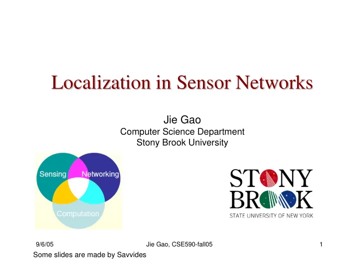
Localization in Sensor Networks Localization in Sensor Networks Jie Gao Computer Science Department Stony Brook University 9/6/05 Jie Gao, CSE590-fall05 1 Some slides are made by Savvides

Find where the sensor is… Find where the sensor is… • Location information is important. 1. Devices need to know where they are. • Sensor tasking: turn on the sensor near the window… 2. We want to know where the data is about. • A sensor reading is too hot – where? 3. It helps infrastructure establishment, such as geographical routing and sensor coverage. • Intruder detection; • Localized geographical routing. 9/6/05 Jie Gao, CSE590-fall05 2

GPS is not always good GPS is not always good • Requires clear sky, doesn’t work indoor. • Too expensive. – A $1 sensor attached with a $100 GPS? Localization: • (optional) Some nodes (anchors or beacons) have GPS or know their locations. • Nodes make local measurements; – Distances between two sensors, angles between two neighbors, etc. • Communicate between each other; • Infer location information from these measurements. 9/6/05 Jie Gao, CSE590-fall05 3

Model of a sensor network Model of a sensor network • Sensor networks with omni-directional antennas are usually modeled by unit disk graphs. – Two nodes have a link if and only if their distance is within 1. • Use the graph property (connectivity, local measurements) to deduct the locations. 9/6/05 Jie Gao, CSE590-fall05 4

Localization problem Localization problem • Output: nodes’ location. – Global location, e.g., what GPS gives. – Relative location. • Input: – Connectivity, hop count. • Nodes with k hops away are within Euclidean distance k. • Nodes without a link must be at least distance 1 away. – Distance measurement of an incoming link. – Angle measurement of an incoming link. – Combinations of the above. 9/6/05 Jie Gao, CSE590-fall05 5

Measurements Measurements Distance estimation: • Received Signal Strength Indicator (RSSI) – The further away, the weaker the received signal. – Mainly used for RF signals. • Time of Arrival (ToA) or Time Difference of Arrival (TDoA) – Signal propagation time translates to distance. – RF, acoustic, infrared and ultrasound. Angle estimation: • Angle of Arrival (AoA) – Determining the direction of propagation of a radio-frequency wave incident on an antenna array. • Directional Antenna • Special hardware, e.g., laser transmitter and receivers. 9/6/05 Jie Gao, CSE590-fall05 6

Localization Localization • Given distances or angle measurements, find the locations of the sensors. • Anchor-based – Some nodes know their locations, either by a GPS or as pre- specified. • Anchor-free – Relative location only. – A harder problem, need to solve the global structure. Nowhere to start. • Range-based – Use range information (distance estimation). • Range-free – No distance estimation, use connectivity information such as hop count. 9/6/05 Jie Gao, CSE590-fall05 7

Many ways to approach this problem Many ways to approach this problem • Trilateration and triangulation • Fingerprinting and classification • Ad-hoc and range/free • Graph rigidity • Identifying codes • Bayesian Networks • Optimization • Multi-dimensional scaling 9/6/05 Jie Gao, CSE590-fall05 8

Trilateration and Triangulation and Triangulation Trilateration • Use geometry, measure the distances/angles to three anchors. • Trilateration: use distances – Global Positioning System (GPS) • Triangulation: use angles – Cell phone systems. • How to deal with inaccurate measurements? • How to solve for more than 3 (inaccurate) measurements? 9/6/05 Jie Gao, CSE590-fall05 9

Ad- -hoc approaches hoc approaches Ad • Ad-hoc positioning (APS) – Estimate range to landmarks using hop count or distance summaries • APS: – Count hops between landmarks – Find average distance per hop – Use multi-lateration to compute location 9/6/05 Jie Gao, CSE590-fall05 10

Optimization Optimization • View system of nodes, distances and angles as a system of equation with unknowns. • Add inequalities – E.g. radio range is at most 1. • Solve resulting system of inequalities as an optimization problem. 9/6/05 Jie Gao, CSE590-fall05 11

Multidimensional Scaling (MDS) Multidimensional Scaling (MDS) • MDS is a general method of finding points in a geometric space that preserves the pair-wise distances as much as possible. – It works also for non-metric data. • Given the pairwise distances P, find a set of points X in m-dimensional space. • Take the largest 2 eigenvalues and eigenvectors of X as the best 2D approximations. 9/6/05 Jie Gao, CSE590-fall05 12

Fingerprinting, classification and scene Fingerprinting, classification and scene analysis analysis • Offline phase: collect training data (fingerprints): [(x, y), SS]. [(x,y),s1,s2,s3] – E.g., the mean Signal Strength to N landmarks. RSS • Online phase: Match RSS to existing fingerprints probabilistically or by [-80,-67,-50] using a distance metric. • Cons: (x?,y?) – How to build the map? • Someone walks around and [(x,y),s1,s2,s3] samples? [(x,y),s1,s2,s3] • Automatic? – Sampling rate? – Changes in the scene (people moving around in a building) affect the signal strengths. 9/6/05 Jie Gao, CSE590-fall05 13

Bayesian Networks Bayesian Networks • View positions as random variables • Build network to describe likely values of these variables given observations • Pros: – Captures any set of observations and priors • Cons: – Computationally expensive – Accuracy 9/6/05 Jie Gao, CSE590-fall05 14

Papers Papers • Multi-lateration: • [Savvides01] A. Savvides, C.-C. Han, and M. B. Strivastava. Dynamic fine-grained localization in ad-hoc networks of sensors . Proc. MobiCom 2001. • [Savvides03] A. Savvides, H. Park, and M. B. Strivastava. The n -hop multilateration primitive for node localization problems , Mobile Networks and Applications, Volume 8, Issue 4, 443-451, 2003. • Mass-spring model: • [Howard01] A. Howard, M. J. Mataric, and G. Sukhatme, Relaxation on a Mesh: a Formalism for Generalized Localization , IEEE/RSJ Internaltionsl Conference on Intelligent Robots and Systems, October, 2001. 9/6/05 Jie Gao, CSE590-fall05 15

Multilateration: use plane geometry : use plane geometry Multilateration 9/6/05 Jie Gao, CSE590-fall05 16

Base Case: Atomic Multilateration Multilateration Base Case: Atomic Base Station 1 u Base Station 3 Base Station 2 • Base stations advertise their coordinates & transmit a reference signal • PDA uses the reference signal to estimate distances to each of the base stations 9/6/05 Jie Gao, CSE590-fall05 17

Base Case: Atomic Multilateration Multilateration Base Case: Atomic • Distance measurements are noisy! • Solve an optimization problem: minimize the mean square error. 9/6/05 Jie Gao, CSE590-fall05 18

Problem Formulation Problem Formulation ( x i y , ) • k beacons at positions i ( x 0 y , ) • Assume node 0 has position 0 • Distance measurement between node 0 and r beacon i is i • Error: 2 2 = − − + − f r ( x x ) ( y y ) i i i 0 i 0 • The objective function is � 2 = F x y ( , ) min f 0 0 i • This is a non-linear optimization problem 9/6/05 Jie Gao, CSE590-fall05 19

Linearization and Min Mean Square Min Mean Square Linearization and Estimate Estimate • Ideally, we would like the error to be 0 2 2 = − − + − = f r ( x x ) ( y y ) 0 i i i 0 i 0 • Re-arrange: 2 2 2 2 2 + + − + − − = − − ( x y ) x ( 2 ) x y ( 2 y ) r x y 0 0 0 i 0 i i i i • Subtract the last equation from the previous ones to get rid of quadratic terms. 2 2 2 2 2 2 − + − = − − − + + 2 x ( x x ) 2 y ( y y ) r r x y x y 0 k i 0 k i i k i i k k • Note that this is linear. 9/6/05 Jie Gao, CSE590-fall05 20

Linearization and Min Mean Square Min Mean Square Linearization and Estimate Estimate • In general, we have an over-constrained linear system = Ax b � � 2 2 2 2 2 2 − − − + + r r x y x y � � − − 2( x x ) 2( y y ) 1 k 1 1 k k � � k 1 k 1 � � 2 2 2 2 2 2 − − − + + r r x y x y � � − − 2( ) 2( ) x x y y = � � � 2 k 2 2 k k = � b k 2 k 2 A � � � � � � � � � � � � � 2 2 2 2 2 2 � − − � � − − − + + � 2( x x ) 2( y y ) r r x y x y − − k k 1 k k 1 − − − k 1 k k 1 k 1 k k � � x = � 0 � x A x = b � � y 0 9/6/05 Jie Gao, CSE590-fall05 21

Solve using the Least Square Solve using the Least Square Equation Equation The linearized equations in matrix form become = Ax b Now we can use the least squares equation to compute an estimation. T − 1 T = x ( A A ) A b 9/6/05 Jie Gao, CSE590-fall05 22