Linear Regression An Error Function: Least Squared Error } For a - PowerPoint PPT Presentation

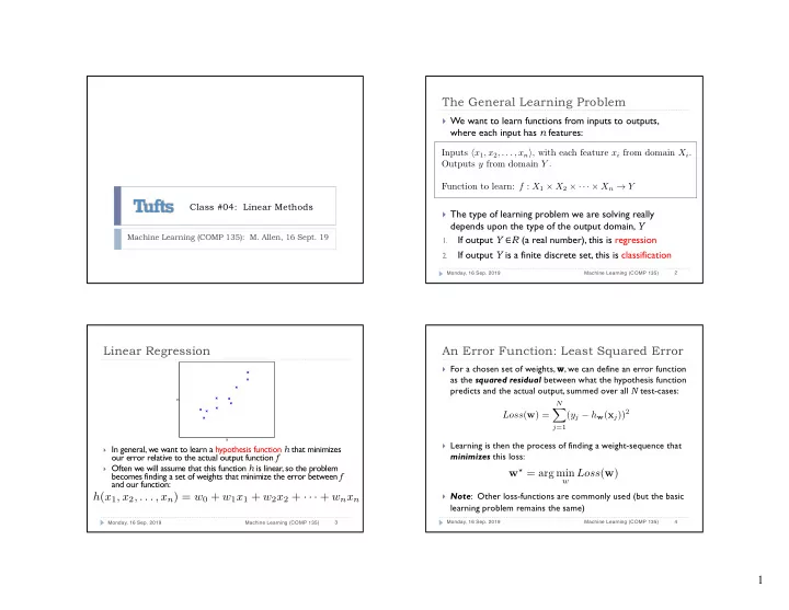
The General Learning Problem } We want to learn functions from inputs to outputs, where each input has n features: Inputs h x 1 , x 2 , . . . , x n i , with each feature x i from domain X i . Outputs y from domain Y . Function to learn: f : X 1 ⇥ X 2 ⇥ · · · ⇥ X n ! Y Class #04: Linear Methods } The type of learning problem we are solving really depends upon the type of the output domain, Y Machine Learning (COMP 135): M. Allen, 16 Sept. 19 If output Y ∈ R (a real number) , this is regression 1. If output Y is a finite discrete set, this is classification 2. 2 Monday, 16 Sep. 2019 Machine Learning (COMP 135) Linear Regression An Error Function: Least Squared Error } For a chosen set of weights, w , we can define an error function as the squared residual between what the hypothesis function predicts and the actual output, summed over all N test-cases: y N X ( y j − h w ( x j )) 2 Loss ( w ) = j =1 x } Learning is then the process of finding a weight-sequence that } In general, we want to learn a hypothesis function h that minimizes minimizes this loss: our error relative to the actual output function f } Often we will assume that this function h is linear, so the problem w ? = arg min w Loss ( w ) becomes finding a set of weights that minimize the error between f and our function: } Note : Other loss-functions are commonly used (but the basic h ( x 1 , x 2 , . . . , x n ) = w 0 + w 1 x 1 + w 2 x 2 + · · · + w n x n learning problem remains the same) 4 Monday, 16 Sep. 2019 Machine Learning (COMP 135) 3 Monday, 16 Sep. 2019 Machine Learning (COMP 135) 1

<latexit sha1_base64="9+1uaXVEozFi2/1CVduDzrznNjI=">ACLnicZVDLTsJAFJ3iCxW16tLNRGMCUmLC10S3chOExESprpdEpHp1meisSwlf4Ifol7jQx8bH1MxAF8hNZnLmzLmv4yWCp2BZb0Zubn5hcSm/vLJaWFvfMDe3blKZKcrqVAqpmh5JmeAxqwMHwZqJYiTyBGt43fPRf+OqZTL+Br6CWtHpBPzgFMCmnLNWs+1sIMdwQIgSsmefoyoA+wQkYQEO2kWube42NfXEQ5dJyIQesGgNyz+wfuhe1squeaeVbGgWeB/Qv2qrWH9+pSo3Dpms+OL2kWsRioIGnasq0E2gOigFPBhitOlrKE0C7psMF40SHe15SPA6n0iQGP2SldLG82FR2K4PgtD3gcZIBi+mkTJAJDBKPME+V4yC6GtAqOK6P6YhUYSCdm6qksoE8w/x3chuX8qOlLrw6i59UG2P/XnQU3lbJ9XK5caSfO0CTyaAftoiKy0Qmqogt0ieqIokf0gj7Rl/FkvBofxtdEmjN+c7bRVBjfP32tqhA=</latexit> <latexit sha1_base64="UNINs4PSoyLlMZSJoJr3l+I7nM=">ACB3icZVBLT8JAGNziC8FH1aOXDWgCiZIWD3okevGIiTwSIM12u4WFbfZblFCetc/ozfkarx794fo2aXgAZlk8ns95hv7IDRUBrGl5ZaW9/Y3EpvZ7I7u3v7+sFhPeSRwKSGOeOiaOQMOqTmqSkWYgCPJsRhr24Gb23xgSEVLu38tRQDoe6vrUpRhJVl6rjCy+vAc9qy2h2TPdscPceGPsZWv1i09LxRMhLAVWIuSL5y8j35GZ/qpb+2XY4jziS8xQGLZMI5CdMRKSYkbiTDsKSYDwAHXJOLkghqdKcqDLhXq+hIm6VOdzmThe6m5F0r3qjKkfRJL4eD7GjRiUHM6OhQ4VBEs2UgRhQdV+iHtICxVJEuTRMSIcwaHsxwd5ZV1uarveWXlVwVg/j93ldTLJfOiVL5TSVyDOdLgGORAZjgElTALaiCGsDgCbyANzDVnrVXbaJN56UpbdFzBJagvf8CzfmdNA=</latexit> An Example Finding Minimal-Error Weights w ? = arg min w Loss ( w ) We can in principle solve for the weight with least error analytically } Create data matrix with one training input example per row, one feature per 1. column, and output vector of all training outputs y     f 11 f 12 f 1 n y 1 · · · f 21 f 22 f 2 n y 2 · · ·     X = y =     . . . . ...     . . . . . . . .     f N 1 f N 2 f Nn y N · · · x } For the data given, the best fit for a simple linear function Solve for the minimal weights using linear algebra (for large data, requires 2. of x is as follows: optimized routines for finding matrix inverses, doing multiplications, etc., as well as for certain matrix properties to hold, which are not universal): h ( x ) ← − y = 1 . 05 + 1 . 60 x w ? = ( X > X ) � 1 X > y 6 Monday, 16 Sep. 2019 Machine Learning (COMP 135) 5 Monday, 16 Sep. 2019 Machine Learning (COMP 135) Finding Minimal-Error Weights Updating Weights w ? = arg min X w Loss ( w ) w i ← w i + α x j,i ( y j − h w ( x j )) j } Weights that minimize error can instead be found (or at least } For each value i , t he update equation takes into account: approximated) using gradient descent: The current weight-value, w i 1. Loop repeatedly over all weights w i , updating them based on their 1. The difference (positive or negative) between the current 2. “contribution” to the overall error: hypothesis for input j and the known output: ( y j − h w ( x j )) X The i -th feature of the data, x j,i w i ← w i + α x j,i ( y j − h w ( x j )) 3. } When doing this update, we must remember that for n data j features, we have ( n + 1) weights, including the bias, w 0 Learning rate : multiplying Feature : normalized Overall Error : difference h ( x 1 , x 2 , . . . , x n ) = w 0 + w 1 x 1 + w 2 x 2 + · · · + w n x n parameter for weight value of feature i of between current and correct training input j outputs for case j adjustments } It is presumed that the related “feature” x j, 0 = 1 in every case, and so the update for the bias weight becomes: Stop on convergence , when maximum update on any weight ( D ) drops 2. below some threshold ( Q ) ; alternatively, stop when change in error/loss X w 0 ← w 0 + α ( y j − h w ( x j )) grows small enough j 8 Monday, 16 Sep. 2019 Machine Learning (COMP 135) 7 Monday, 16 Sep. 2019 Machine Learning (COMP 135) 2