Linear Regression 4/14/17 Hypothesis Space Supervised learning - PowerPoint PPT Presentation
Linear Regression 4/14/17 Hypothesis Space Supervised learning For every input in the data set, we know the output Regression Outputs are continuous A number, not a category label The learned model: A linear function mapping
Linear Regression 4/14/17
Hypothesis Space Supervised learning • For every input in the data set, we know the output Regression • Outputs are continuous • A number, not a category label The learned model: • A linear function mapping input to output • A weight for each feature (including bias)
Linear Models In two dimensions: f ( x ) = wx + b In d dimensions: 1 w b x 0 w 0 x 0 x 1 f ( ~ x ) = ~ . . x ≡ · . . . . . . . w d x d x d We want to find the linear model that fits our data best. When have we seen a model like this before?
Linear Regression We want to find the linear model that fits our data best. Key idea: model data as linear model plus noise. Pick the weights to minimize noise magnitude. 1 w b w 0 x 0 f ( ~ x ) = + ✏ . . · . . . . w d x d
Squared Error 1 1 w b w b w 0 x 0 w 0 x 0 ˆ f ( ~ x ) = + ✏ f ( ~ x ) = . . . . · · . . . . . . . . w d x d w d x d Define error for a data point to be the squared distance between correct output and predicted output: ⌘ 2 ⇣ x ) − ˆ = ✏ 2 f ( ~ f ( ~ x ) Error for the model is the sum of point errors: ⇣ ⌘ y − ˆ X X ✏ 2 f ( ~ x ) = ~ x ~ x ∈ data ~ x ∈ data
Minimizing Squared Error Goal: pick weights that minimize squared error. Approach #1: gradient descent Your reading showed how to do this for 1D inputs:
Minimizing Squared Error Goal: pick weights that minimize squared error. Approach #2 (the right way): analytical solution • The gradient is 0 at the error minimum. • There is generally a unique global minimum. ⌘ − 1 ⇣ X T X X T ~ ~ w = y 2 3 1 1 1 . . . x 00 x 01 . . . x 0 n 6 7 6 7 ⇥ ~ ⇤ x 10 x 11 . . . x 1 n x 1 . . . ~ ~ X ≡ 6 7 x 0 x n ≡ 6 7 . . . ... . . . 6 7 . . . 4 5 x d 0 x d 1 . . . x dn
Change of Basis Polynomial regression is just linear regression with a change of basis. cubic x 0 basis ( x 0 ) 2 quadratic x 0 ( x 0 ) 3 basis ( x 0 ) 2 x 0 x 1 x 0 x 1 ( x 1 ) 2 x 1 x 1 ( x 1 ) 2 . ( x 1 ) 3 . − → − → . . . . . . . . . . x d x d x d x d ( x d ) 2 ( x d ) 2 ( x d ) 3 Perform linear regression on the new representation.
Change of Basis Demo
Locally Weighted Regression Recall from KNN: locally weighted averaging We can apply the same idea here: points that are further away should contribute less to the estimate. To estimate the value for a specific test point x t compute a linear regression with error weighted by distance: ⇣ ⌘ y − ˆ f ( ~ x ) ✏ 2 X X ~ x x ) = dist ( ~ || ~ x || 2 x t , ~ x t − ~ x ∈ data ~ ~ x ∈ data
Exam Topics Covers the machine learning portion of the class. • Supervised learning • Regression • Classification • Unsupervised learning • Clustering • Dimensionality reduction • Semi-supervised learning • Reinforcement learning Know the differences between these topics. Know what algorithms apply to which problems.
Machine Learning Algorithms • neural networks • EM • perceptrons • K-means • backpropagation • Gaussian mixtures • auto-encoders • hierarchical clustering • deep learning • agglomerative • decision trees • divisive • naive Bayes • principal component analysis • k-nearest neighbors • growing neural gas • support vector machines • Q-learning • locally-weighted average • approximate Q-learning • linear regression • ensemble learning
Recommend
More recommend
Explore More Topics
Stay informed with curated content and fresh updates.
