Linear Regression 18.05 Spring 2014 Jeremy Orloff and Jonathan Bloom - PowerPoint PPT Presentation

Linear Regression 18.05 Spring 2014 Jeremy Orloff and Jonathan Bloom

Agenda Fitting curves to bivariate data Measuring the goodness of fit The fit vs. complexity tradeoff Multiple linear regression June 10, 2014 2 / 17

Modeling bivariate data as a function + noise Ingredients Bivariate data ( x 1 , y 1 ) , ( x 2 , y 2 ) , . . . , ( x n , y n ) . Model: y i = f ( x i ) + E i f ( x ) some function, E i random error. Total squared error: n n n 2 = ( y i − f ( x i )) 2 n E i i =1 i =1 With a model we can predict the value of y for any given value of x . x is called the independent or predictor variable . y is the dependent or response variable. June 10, 2014 3 / 17

Examples lines: y = ax + b + E polynomials: y = ax 2 + bx + c + E other: y = a / x + b + E other: y = a sin ( x ) + b + E June 10, 2014 4 / 17

Simple linear regression: finding the best fitting line Bivariate data ( x 1 , y 1 ) , . . . , ( x n , y n ). Simple linear regression: fit a line to the data y i = ax i + b + E i , where E i ∼ N(0 , σ 2 ) and where σ is a fixed value, the same for all data points. n n n n 2 = ( y i − ax i − b ) 2 Total squared error: E i i =1 i =1 Goal: Find the values of a and b that give the ‘best fitting line’. Best fit: ( least squares ) The values of a and b that minimize the total squared error. June 10, 2014 5 / 17

Linear Regression: finding the best fitting polynomial Bivariate data: ( x 1 , y 1 ) , . . . , ( x n , y n ). Linear regression: fit a parabola to the data 2 + bx i + c + E i , where E i ∼ N(0 , σ 2 ) y i = ax i and where σ is a fixed value, the same for all data points. n n n 2 = 2 − bx i − c ) 2 . n Total squared error: ( y i − ax i E i i =1 i =1 Goal: Find the values of a , b , c that give the ‘best fitting parabola’. Best fit: ( least squares ) The values of a , b , c that minimize the total squared error. Can also fit higher order polynomials. June 10, 2014 6 / 17

Stamps Stamp cost (cents) vs. time (years since 1960) (Red dot is predicted cost in 2015.) June 10, 2014 7 / 17

Parabolic fit 15 10 y 5 0 −1 1 2 3 4 5 6 x June 10, 2014 8 / 17 a

Board question: make it fit Bivariate data: (1 , 3) , (2 , 1) , (4 , 4) 1. Do (simple) linear regression to find the best fitting line. Hint: minimize the total squared error by taking partial derivatives with respect to a and b . 2. Do linear regression to find the best fitting parabola. 3. Set up the linear regression to find the best fitting cubic. but don’t take derivatives. 4. Find the best fitting exponential y = e ax + b . Hint: take ln( y ) and do simple linear regression. June 10, 2014 9 / 17

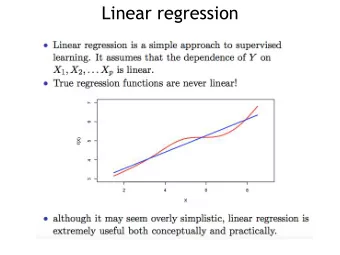
What is linear about linear regression? Linear in the parameters a , b , . . . . y = ax + b . 2 + bx + c . y = ax It is not because the curve being fit has to be a straight line –although this is the simplest and most common case. Notice: in the board question you had to solve a system of simultaneous linear equations . June 10, 2014 10 / 17

Homoscedastic BIG ASSUMPTION in least squares: the E i are independent with the same variance σ . Regression line (left) and residuals (right). Note the homoscedasticity. June 10, 2014 11 / 17

Heteroscedastic Heteroscedastic Data June 10, 2014 12 / 17

Measuring the fit and overfitting y = ( y 1 , · · · , y n ) = data values of the response variable. ˆ = (ˆ y 1 , · · · , y ˆ n ) = ‘fitted values’ of the response variable. y ˆ i = ax i + b y The R 2 measure of goodness-of-fit is given by R 2 = Cor( y , y ˆ) 2 R 2 is the fraction of the variance of y explained by the model. y and R 2 = 1. If all the data points lie on the curve, then y = ˆ (R demonstration right here.) June 10, 2014 13 / 17

Formulas for simple linear regression Model: y i = ax i + b + E i where E i ∼ N(0 , σ 2 ) . Using calculus or algebra: s xy ˆ a = and b = ¯ y − ˆ a ¯ x , ˆ s xx where n n 1 s xx = 1 x ) 2 x = ( x i − ¯ ¯ x i ( n − 1) n n n 1 1 y = ( n − 1) s xy = ( n − 1) ( x i − ¯ x )( y i − ¯ y ). ¯ y i WARNING: This is just for simple linear regression. For polynomials and other functions you need other formulas. June 10, 2014 14 / 17

Board Question: using the formulas plus some theory Bivariate data: (1 , 3) , (2 , 1) , (4 , 4) 1.(a) Calculate the sample means for x and y . 1.(b) Use the formulas to find a best-fit line in the xy -plane. s xy a = b = y − ax ˆ s xx n 1 1 n ( x i − x ) 2 . ( x i − x )( y i − y ) s xx = s xy = n − 1 n − 1 2. Show the point ( x , y ) is always on the fitted line. 3. Under the assumption E i ∼ N(0 , σ 2 ) show that the least squares method is equivalent to finding the MLE for the parameters ( a , b ). Hint: f ( y i | x i , a , b ) ∼ N( ax i + b , σ 2 ). June 10, 2014 15 / 17

Regression to the mean Suppose a group of children is given an IQ test at age 4. One year later the same children are given another IQ test. Children’s IQ scores at age 4 and age 5 should be positively correlated. Those who did poorly on the first test (e.g., bottom 10%) will tend to show improvement (i.e. regress to the mean) on the second test. A completely useless intervention with the poor-performing children might be misinterpreted as causing an increase in their scores. Conversely, a reward for the top-performing children might be misinterpreted as causing a decrease in their scores. This example is from Rice Mathematical Statistics and Data Analysis June 10, 2014 16 / 17

A brief discussion of multiple linear regression Multivariate data: ( x i , 1 , x i , 2 , . . . , x i , m , y i ) ( n data points: i = 1 , . . . , n ) Model ˆ y i = a 1 x i , 1 + a 2 x i , 2 + . . . + a m x i , m x i , j are the explanatory (or predictor) variables. y i is the response variable. The total squared error is n n n ˆ i ) 2 = ( y i − a 1 x i , 1 − a 2 x i , 2 − . . . − a m x i , m ) 2 n ( y i − y i =1 i =1 June 10, 2014 17 / 17

MIT OpenCourseWare http://ocw.mit.edu 18.05 Introduction to Probability and Statistics Spring 2014 For information about citing these materials or our Terms of Use, visit: http://ocw.mit.edu/terms.