Linear Regression 18.05 Spring 2018 Agenda Fitting curves to - PowerPoint PPT Presentation
Linear Regression 18.05 Spring 2018 Agenda Fitting curves to bivariate data Measuring the goodness of fit The fit vs. complexity tradeoff Regression to the mean Multiple linear regression May 13, 2018 2 / 24 Modeling bivariate data as a
Linear Regression 18.05 Spring 2018
Agenda Fitting curves to bivariate data Measuring the goodness of fit The fit vs. complexity tradeoff Regression to the mean Multiple linear regression May 13, 2018 2 / 24
Modeling bivariate data as a function + noise Ingredients Bivariate data ( x 1 , y 1 ) , ( x 2 , y 2 ) , . . . , ( x n , y n ) . Model: y i = f ( x i ) + E i where f ( x ) is a function we pick (the model), E i random error. n n � � E 2 ( y i − f ( x i )) 2 Total squared error: i = i =1 i =1 Model predicts the value of y for any given value of x . • x is called the independent or predictor variable. • y is the dependent or response variable. • Error from imperfect model, or imperfect measurement, or. . . May 13, 2018 3 / 24
Examples of f ( x ) lines: y = ax + b + E polynomials: y = ax 2 + bx + c + E other: y = a / x + b + E other: y = a sin( x ) + b + E May 13, 2018 4 / 24
Simple linear regression: finding the best fitting line Bivariate data ( x 1 , y 1 ) , . . . , ( x n , y n ). Simple linear regression: fit a line to the data where E i ∼ N(0 , σ 2 ) y i = ax i + b + E i , and where σ is a fixed value, the same for all data points. n n � � E 2 ( y i − ax i − b ) 2 Total squared error: = i i =1 i =1 Goal: Find the values of a and b that give the ‘best fitting line’. Best fit: (least squares) The values of a and b that minimize the total squared error. May 13, 2018 5 / 24
Linear Regression: finding the best fitting polynomial Bivariate data: ( x 1 , y 1 ) , . . . , ( x n , y n ). Linear regression: fit a parabola to the data y i = ax 2 where E i ∼ N(0 , σ 2 ) i + bx i + c + E i , and where σ is a fixed value, the same for all data points. n n � E 2 � ( y i − ax 2 i − bx i − c ) 2 . Total squared error: = i i =1 i =1 Goal: Find a , b , c giving the ‘best fitting parabola’. Best fit: (least squares) The values of a , b , c that minimize the total squared error. May 13, 2018 6 / 24
Stamps 50 ● ● ● ● ● ● 40 ● ● ● ● ● ● 30 ● y ● ● 20 ● ● ● 10 ● ● ● ● 0 10 20 30 40 50 60 x Stamp cost (cents) vs. time (years since 1960) (Red dot = 49 cents is predicted cost in 2016.) (Actual cost of a stamp dropped from 49 to 47 cents on 4/8/16.) May 13, 2018 7 / 24
Parabolic fit 15 10 y 5 0 −1 0 1 2 3 4 5 6 x May 13, 2018 8 / 24
Board question: make it fit Bivariate data: (1 , 3) , (2 , 1) , (4 , 4) 1. Do (simple) linear regression to find the best fitting line. Hint: minimize the total squared error by taking partial derivatives with respect to a and b . 2. Do linear regression to find the best fitting parabola. 3. Set up the linear regression to find the best fitting cubic. but don’t take derivatives. 4. Find the best fitting exponential y = e ax + b . Hint: take ln( y ) and do simple linear regression. May 13, 2018 9 / 24
Solutions 1. Model ˆ y i = ax i + b . � y i ) 2 total squared error = T = ( y i − ˆ � ( y i − ax i − b ) 2 = = (3 − a − b ) 2 + (1 − 2 a − b ) 2 + (4 − 4 a − b ) 2 Take the partial derivatives and set to 0: ∂ T = − 2(3 − a − b ) − 4(1 − 2 a − b ) − 8(4 − 4 a − b ) = 0 ∂ a ∂ T = − 2(3 − a − b ) − 2(1 − 2 a − b ) − 2(4 − 4 a − b ) = 0 ∂ b A little arithmetic gives the system of simultaneous linear equations and solution: 42 a +14 b = 42 ⇒ a = 1 / 2 , b = 3 / 2 . 14 a +6 b = 16 The least squares best fitting line is y = 1 2 x + 3 2. May 13, 2018 10 / 24
Solutions continued y i = ax 2 2. Model ˆ i + bx i + c . Total squared error: � y i ) 2 T = ( y i − ˆ � ( y i − ax 2 i − bx i − c ) 2 = = (3 − a − b − c ) 2 + (1 − 4 a − 2 b − c ) 2 + (4 − 16 a − 4 b − c ) 2 We didn’t really expect people to carry this all the way out by hand. If you did you would have found that taking the partial derivatives and setting to 0 gives the following system of simultaneous linear equations. 273 a +73 b +21 c = 71 73 a +21 b +7 c = 21 ⇒ a = 1 . 1667 , b = − 5 . 5 , c = 7 . 3333 . 21 a +7 b +3 c = 8 The least squares best fitting parabola is y = 1 . 1667 x 2 + − 5 . 5 x + 7 . 3333. May 13, 2018 11 / 24
Solutions continued y i = ax 3 i + bx 2 3. Model ˆ i + cx i + d . Total squared error: y i ) 2 � T = ( y i − ˆ � ( y i − ax 3 i − bx 2 i − cx i − d ) 2 = = (3 − a − b − c − d ) 2 + (1 − 8 a − 4 b − 2 c − d ) 2 + (4 − 64 a − 16 b − 4 c In this case with only 3 points, there are actually many cubics that go through all the points exactly. We are probably overfitting our data. y i = e ax i + b 4. Model ˆ ⇔ ln( y i ) = ax i + b . Total squared error: � y i )) 2 T = (ln( y i ) − ln(ˆ � (ln( y i ) − ax i − b ) 2 = = (ln(3) − a − b ) 2 + (ln(1) − 2 a − b ) 2 + (ln(4) − 4 a − b ) 2 Now we can find a and b as before. (Using R: a = 0 . 18, b = 0 . 41) May 13, 2018 12 / 24
What is linear about linear regression? Linear in the parameters a , b , . . . . y = ax + b . y = ax 2 + bx + c . It is not because the curve being fit has to be a straight line –although this is the simplest and most common case. Notice: in the board question you had to solve a system of simultaneous linear equations. Fitting a line is called simple linear regression. May 13, 2018 13 / 24
Homoscedastic BIG ASSUMPTIONS : the E i are independent with the same variance σ 2 . 20 ● ● ● ● ● ● ● ● ● ● ● ● ● ● 15 ● ● ● ● ● ● ● ● ● ● ● ● ● ● ● ● ● ● ● ● ● ● ● ● ● ● ● ● ● ● ● ● ● 10 ● ● ● ● ● ● y ● ● ● ● ● ● ● ● ● ● ● ● ● ● ● ● ● ● ● ● ● ● ● ● ● ● ● ● ● ● ● ● ● ● 5 ● ● ● ● ● ● ● ● ● ● ● ● ● ● 0 0 2 4 6 8 10 x ● 4 ● 3 ● ● ● ● ● ● ● 2 ● ● ● ● ● ● ● ● ● ● ● ● ● ● ● 1 ● ● ● ● ● ● e ● ● ● ● ● ● ● ● ● ● ● ● ● ● ● ● ● ● ● ● ● ● ● ● 0 ● ● ● ● ● ● ● ● ● ● ● ● ● ● ● ● ● ● May 13, 2018 14 / 24 ● ● ● ● ● −1 ● ● ● ● ●
Heteroscedastic 20 ● ● ● ● ● ● ● ● ● ● ● ● 15 ● ● ● ● ● ● ● ● ● ● ● ● ● ● ● ● ● ● ● ● ● ● ● ● ● ● ● ● ● ● ● ● ● ● ● ● ● ● ● ● ● ● ● ● ● ● ● ● ● ● 10 ● ● ● ● ● ● y ● ● ● ● ● ● ● ● ● ● ● ● ● ● ● ● ● ● ● ● ● ● ● ● ● ● ● ● ● ● ● ● ● ● ● ● ● ● ● ● ● ● ● ● ● ● ● 5 ● ● ● ● ● ● ● ● ● ● ● ● ● ● ● ● ● ● ● ● ● ● ● ● ● ● ● ● 0 0 2 4 6 8 10 x Heteroscedastic Data May 13, 2018 15 / 24
Formulas for simple linear regression Model: y i = ax i + b + E i where E i ∼ N(0 , σ 2 ) . Using calculus or algebra: a = s xy ˆ ˆ and b = ¯ y − ˆ a ¯ x , s xx where x = 1 1 � � x ) 2 ¯ x i s xx = ( x i − ¯ n n − 1 y = 1 1 � � ¯ s xy = ( x i − ¯ x )( y i − ¯ y ). y i n − 1 n WARNING: This is just for simple linear regression. For polynomials and other functions you need other formulas. May 13, 2018 16 / 24
Board Question: using the formulas plus some theory Bivariate data: (1 , 3) , (2 , 1) , (4 , 4) 1.(a) Calculate the sample means for x and y . 1.(b) Use the formulas to find a best-fit line in the xy -plane. a = s xy ˆ ˆ b = y − ˆ ax s xx 1 1 � � ( x i − x ) 2 . s xy = ( x i − x )( y i − y ) s xx = n − 1 n − 1 2. Show the point ( x , y ) is always on the fitted line. 3. Under the assumption E i ∼ N(0 , σ 2 ) show that the least squares method is equivalent to finding the MLE for the parameters ( a , b ). Hint: f ( y i | x i , a , b ) ∼ N( ax i + b , σ 2 ). May 13, 2018 17 / 24
Solution answer: 1. (a) ¯ x = 7 / 3, ¯ y = 8 / 3. (b) s xx = (1 + 4 + 16) / 3 − 49 / 9 = 14 / 9 , s xy = (3 + 2 + 16) / 3 − 56 / 9 = 7 / 9 . So a = s xy ˆ ˆ = 7 / 14 = 1 / 2 , b = ¯ y − ˆ a ¯ x = 9 / 6 = 3 / 2 . s xx (The same answer as the previous board question.) 2. The formula ˆ x + ˆ b = ¯ y − ˆ a ¯ x is exactly the same as ¯ y = ˆ a ¯ b . That is, ax + ˆ the point (¯ x , ¯ y ) is on the line y = ˆ b Solution to 3 is on the next slide. May 13, 2018 18 / 24
3. Our model is y i = ax i + b + E i , where the E i are independent. Since E i ∼ N(0 , σ 2 ) this becomes y i ∼ N( ax i + b , σ 2 ) Therefore the likelihood of y i given x i , a and b is e − ( yi − axi − b )2 1 f ( y i | x i , a , b ) = √ 2 σ 2 2 πσ Since the data y i are independent the likelihood function is just the product of the expression above, i.e. we have to sum exponents i =1( yi − axi − b )2 � n likelihood = f ( y 1 , . . . , y n | x 1 , . . . , x n , a , b ) = e − 2 σ 2 Since the exponent is negative, the maximum likelihood will happen when the exponent is as close to 0 as possible. That is, when the sum n � ( y i − ax i − b ) 2 i =1 is as small as possible. This is exactly what we were asked to show. May 13, 2018 19 / 24
Recommend
More recommend
Explore More Topics
Stay informed with curated content and fresh updates.
