Linear Functions and Models Functions and Mathematical Mod- eling - - PDF document

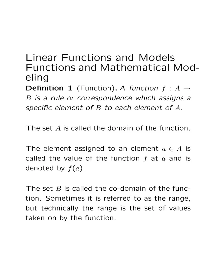
Linear Functions and Models Functions and Mathematical Mod- eling

Definition 1 (Function). A function f : A → B is a rule or correspondence which assigns a specific element of B to each element of A. The set A is called the domain of the function. The element assigned to an element a ∈ A is called the value of the function f at a and is denoted by f(a). The set B is called the co-domain of the func-

• tion. Sometimes it is referred to as the range,

but technically the range is the set of values taken on by the function.

Example: f(x) = x2 or y = x2 These are alternate notations for giving the correspondence defining a function. In each, x is called the independent variable. In the second case, y is called the dependent variable. Everyday functions: Population is a function of time. Postage is a function of weight. The balance in a bank account is a function of time. The area of a circle is a function of its radius. Functions are used to model problems.

Example: Dog pen problem (page 9): A dog pen is to be made from 60 feet of fencing, enclosing three sides of a rectangular region. (The fourth side is an existing wall.) The area

• f the pen can be represented as a function of

the length of the side opposite the wall. Let x be the length (in feet) of the side op- posite the wall. The other two sides, of equal length, have to total 60 − x feet, so each must have length 60−x

2

. If we represent the area by A, we have A = x ·

60−x

2

• .

Problem: Suppose we want the area to be 400 square feet? Solution: Since the area is equal to = x·

60−x

2

• ,

it follows that we need to have x ·

60−x

2

• =

400. We can find the dimensions of the pen by solving this equation.

Linear Functions

A linear function is a function of the form f(x) = mx + b. m is called the slope. b is called the vertical intercept. If the depen- dent variable is y, it is called the y−intercept.

Graphs

The graph of a function f : A → B is {(x, y) : y = f(x)}.

Equations of Lines Slope-Intercept Form

y = mx + b

Point-Slope Form

y − y0 = m(x − x0), where the slope is m and (x0, y0) is a point on the graph.

Linear Growth

We have linear growth when there is a constant rate of change. Linear growth in a population may be modeled with the formula P = P0+mt. Some situations are best modeled by piecewise linear functions, whose graphs are the unions

• f line segments.

Fitting Linear Models to Data

Definition 2 (Average Rate of Change). The average rate of change of a population P is

∆P ∆t , where ∆P is the change in the population

and ∆t is the length of time. An obvious model is to create a linear function which agrees with the first size of the popula- tion and has a slope equal to the average rate

• f change.

Problem: It may not be ideal. It’s reasonable to try to minimize the total er- ror. Problem: Positive and negative errors cancel each other out. Solution: Look at the squares of the errors.

Definition 3 (Sum of Squares of the Errors). SSE = the sum of the squares of the errors at all the data points. Our models will minimize SSE. The computa- tions will be performed by calculators or com- puters. Definition 4 (Average Squared Error). The av- erage squared error is the average of the squares

• f the errors, obtained by dividing SSE by the

number of data points. Definition 5 (Average Error). The average er- ror is defined as the square root of the average squared error. Note: The Average Error, as defined, is not literally the average error.

Regression on a Calculator

Store the t and P values in a table as lists L1 and L2, choosing STAT and then choosing EDIT. Calculate the coefficients in the regression P = P0+mt, displayed on the calculator as y = ax+ b, by choosing STAT, then choosing CALC, then choosing LinReg(ax + b) L1, L2, Y1. To plot the regression line along with the data points, choose the STAT PLOT menu di- rectly from the calculator keypad and set Plot 1 to On. The errors or differences between the actual data values and the values predicted by the linear regression, called residuals, are stored in the LIST menu under the name RESID.

Percentages

Percentages are generally used to describe a rate rather than an absolute amount. One finds an absolute amount by multiplying a rate by another quantity. Examples: Speed is a rate. Distance is average speed × time. Acceleration is a rate (the rate at which speed changes). Speed is average acceleration×time. A sales tax rate is a rate. Sales tax is tax rate× price. Interest rate is a rate. Interest is interest rate× balance.

Percent means per cent or per 100. It is actu- ally away of representing a fraction. 6% means 6 per 100 or 6/100 or 0.06. In Connecticut, the sales tax rate is 6%. It would be equally correct to say the sales tax rate is 6/100, or the sales tax rate is 3/50, or the sales tax rate is 0.06. Party Fun: Get up on a chair during a party and tell everyone the sales tax rate in Connecticut is 3/50.

Caution: When mentioning rates, the word rate is often omitted. Thus, we often say that in Connecticut the sales tax is 6% rather than saying the sales tax rate is 6%. It must be un- derstood, when percent is mentioned, that the figure represents a rate even if the term rate is left unsaid. Thus, while the statements “the sales tax is 6%” and “the sales tax is 3/50” literally mean the same thing, they are under- stood to have different meanings. Let P be the price of an item, r the sales tax rate, C the net cost including sales tax. The sales tax is rP, so the total cost is P + rP (the price plus the sales tax). Since P + rP = P(1 + r), we get the formula C = P(1 + r).

Interest

Interest is similar to sales tax. If interest on a balance P0 was computed once a year at an annual rate r, the interest after a year would be rP0, so the balance P after a year would be P0 + rP0 = P0(1 + r) (the original balance plus the interest), so we’d get P = P0(1 + r). This should look very similar to the formula for net cost including sales tax. After two years, interest would be calculated again. The amount of interest would be r × P0(1+r), so the new balance would be P0(1+ r) + r × P0(1 + r) = P0(1 + r)(1 + r), giving us the balance P = P0(1 + r)2. We can continue indefinitely and find that after t years, the balance will be P = P0(1 + r)t. We have built a mathematical model.

Compound Interest

Suppose that instead of interest being com- puted once per year, it was computed twice per year. Each time, the amount of interest computed would be half the amount it would be had it been computed for a full year. Thus, after a half year, the interest would be 1

2×r×P0,

so the balance would be P = P0 + 1

2 × rP0 =

P0(1 + r

2).

After another half year, we’d get interest in the amount 1

2 × r × P0(1 + r 2) so the balance would

be P0(1 + r

2) + 1 2 × r × P0(1 + r 2) = P0(1 + r 2)2.

After two years, the balance would be P0(1 +

r 2)4.

After t years, the balance would be P = P0(1+

r 2)2t.

If, instead of interest being compounded twice a year, it was compounded n times per year, the balance would be P = P0(1 + r

n)nt.

This is called the Compound Interest Formula.

Continuous Interest

Using the properties of exponents, one may rewrite the Compound Interest Formula P = P0(1 + r

n)nt in the form

P = P0

• (1 + r

n)n/rrt

• r

P = P0

• (1 +

1 n/r)n/r

rt

. When interest is compounded very frequently, the quotient n/r will be very large. It turns out that the larger n/r gets, the closer (1+ 1

n/r)n/r

gets to the number e, and thus the closer P gets to P0ert. This leads to the Continuous Interest Formula: P = P0ert.

The number e is a special mathematical con- stant, which is also the base of the natural logarithm function. A decimal approximation to e is e ≈ 2.7182818. For many purposes, it suffices to know 2 < e < 3, that is, e is between 2 and 3.

Paying Off a Loan

Notation

P Initial loan balance Pn Balance after n months m Monthly payment r Monthly interest rate Note: P = P0 Since the balance Pn after n months will be the balance Pn−1 the month before, less the monthly payment m, plus the interest Pn−1r for

• ne month on the balance the month before,

it follows that Pn = Pn−1 − m + Pn−1r = Pn−1(1 + r) − m. So . . . P1 = P0(1 + r) − m or

P1 = P(1 + r) − m P2 = P1(1+r)−m = (P(1+r)−m)(1+r)−m = P(1 + r)2 − m(1 + r) − m P3 = P2(1 + r) − m = (P(1 + r)2 − m(1 + r) − m)(1 + r) − m = P(1 + r)3 − m(1 + r)2 − m(1 + r) − m Similarly, we get P4 = P(1+r)4 −m(1+r)3 −m(1+r)2 −m(1+ r) − m. We can see the pattern that in general we will get Pn = P(1 + r)n − m(1 + r)n−1 − m(1 + r)n−2 − m(1 + r)n−3 − · · · − m(1 + r) − m or Pn = P(1 + r)n − m(1 + (1 + r) + (1 + r)2 + (1 + r)3 + · · · + (1 + r)n−1).

The expression multiplied by m is in the form 1 + x + x2 + x3 + · · · + xn−1. This leads to the question of whether we can simplify 1 + x + x2 + x3 + · · · + xn−1.

Exploration

Factor 1 − x2 Result: 1 − x2 = (1 − x)(1 + x) Factor 1 − x3 Result: 1 − x3 = (1 − x)(1 + x + x2) Factor 1 − x4 Result: 1 − x4 = (1 − x)(1 + x + x2 + x3) Notice a pattern?

It appears that 1−xn = (1−x)(1+x+x2+x3+· · ·+xn−2+xn−1) This can be verified by multiplying the right hand side out: (1 − x)(1 + x + x2 + x3 + · · · + xn−2 + xn−1) = 1−x+x−x2 +x2 −x3 +x3 −· · ·−xn−2 +xn−2 − xn = 1 − xn. This confirms that factorization of 1 − xn and, dividing both sides by 1 − x yields 1 − xn 1 − x = 1 + x + x2 + x3 + · · · + xn−2 + xn−1. This is the formula we need. Replacing x by 1 + r, we get 1 + (1 + r) + (1 + r)2 + · · · + (1 + r)n−1 = 1 − (1 + r)n 1 − (1 + r) = 1 − (1 + r)n −r = (1 + r)n − 1 r and we then can rewrite

Pn = P(1 + r)n − m(1 + (1 + r) + (1 + r)2 + (1 + r)3 + · · · + (1 + r)n−1) as Pn = P(1 + r)n − m · (1 + r)n − 1 r . Suppose we want to calculate a monthly pay- ment if a loan will be paid off in n months? In that case, Pn will equal 0, so we’ll have P(1 + r)n − m · (1 + r)n − 1 r = 0. We can fairly easily solve this for the monthly payment m. P(1 + r)n = m · (1 + r)n − 1 r Switching sides: m · (1 + r)n − 1 r = P(1 + r)n

m = P(1 + r)n [(1 + r)n − 1]/r m = Pr(1 + r)n (1 + r)n − 1. If we divide both numerator and denominator by (1 + r)n, we get m = Pr 1 − (1 + r)−n. This should make sense, since the numerator is Pr, which is one month’s interest on the origi- nal balance, and the denominator is clearly less than one. Thus the monthly payment will be more than one month’s interest on the original

• balance. This is clearly necessary, since other-

wise the balance would keep growing and the loan would never get paid off.

The larger n is, the closer (1 + r)−n will be to 0, so the closer the denominator will be to 1 and the smaller the monthly payment will be. In other words, stretching out the repayment period results in a lower monthly payment. On the other hand, the larger the monthly in- terest rate r, the larger the numerator Pr is and the larger the monthly payment.