Lecture 8: Heteroskedasticity Causes Consequences Detection - PowerPoint PPT Presentation

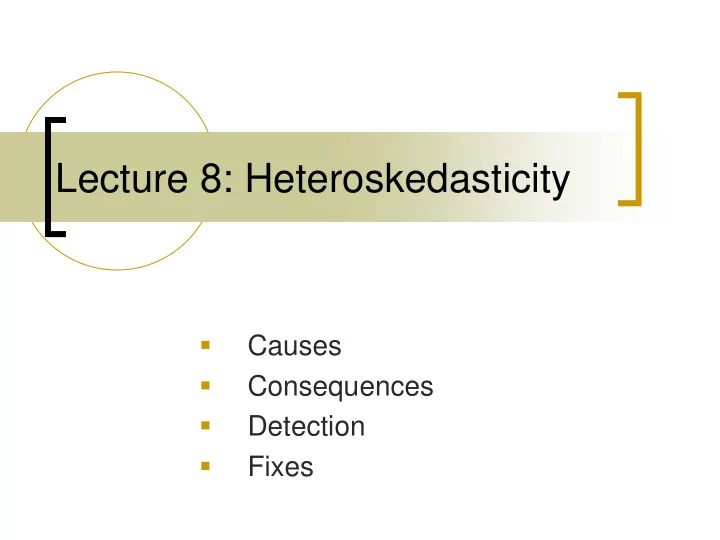
Lecture 8: Heteroskedasticity  Causes  Consequences  Detection  Fixes

Assumption MLR5: Homoskedasticity   2 var( | , ,..., ) u x x x 1 2 j In the multivariate case, this means that the  variance of the error term does not increase or decrease with any of the explanatory variables x 1 through x j . If MLR5 is untrue, we have heteroskedasticity. 

Causes of Heteroskedasticity  Error variance can increase as values of an independent variable increase.  Ex: Regress household security expenditures on household income and other characteristics. Variance in household security expenditures will increase as income increases because you can’t spend a lot on security unless you have a large income.  Error variance can increase with extreme values of an independent variable (either positive or negative)  Measurement error. Extreme values may be wrong, leading to greater error at the extremes.

Causes of Heteroskedasticity, cont.  Bounded independent variable. If Y cannot be above or below certain values, extreme predictions have restricted variance. (See example in 5 th slide after this one.)  Subpopulation differences. If you need to run separate regressions, but run a single one, this can lead to two error distributions and heteroskedasticity.  Model misspecification:  form of included variables (square, log, etc.)  exclusion of relevant variables

Not Consequences of Heteroskedasticity:  MLR5 is not needed to show unbiasedness or consistency of OLS estimates. So violation of MLR5 does not lead to biased estimates.  Since R 2 is based on overall sums of squares, it is unaffected by heteroskedasticity.  Likewise, our estimate of root mean squared error is valid in the presence of heteroskedasticity.

Consequences of heteroskedasticity  OLS model is no longer B.L.U.E. (best linear unbiased estimator)  Other estimators are preferable  With heteroskedasticity, we no longer have the “best” estimator, because error variance is biased.  incorrect standard errors  Invalid t-statistics and F statistics  LM test no longer valid

Detection of heteroskedasticity: graphs  Conceptually, we know that heteroskedasticity means that our predictions have uneven variance over some combination of Xs.  Simple to check in bivariate case, complicated for multivariate models.  One way to visually check for heteroskedasticity is to plot predicted values against residuals  This works for either bivariate or multivariate OLS.  If heteroskedasticity is suspected to derive from a single variable, plot it against the residuals  This is an ad hoc method for getting an intuitive feel for the form of heteroskedasticity in your model

Let’s see if the regression from the 2010 midterm has heteroskedasticity (DV is high school g.p.a.) . reg hsgpa male hisp black other agedol dfreq1 schattach msgpa r_mk income1 antipeer Source | SS df MS Number of obs = 6574 -------------+------------------------------ F( 11, 6562) = 610.44 Model | 1564.98297 11 142.271179 Prob > F = 0.0000 Residual | 1529.3681 6562 .233064325 R-squared = 0.5058 -------------+------------------------------ Adj R-squared = 0.5049 Total | 3094.35107 6573 .470766936 Root MSE = .48277 ------------------------------------------------------------------------------ hsgpa | Coef. Std. Err. t P>|t| [95% Conf. Interval] -------------+---------------------------------------------------------------- male | -.1574331 .0122943 -12.81 0.000 -.181534 -.1333322 hisp | -.0600072 .0174325 -3.44 0.001 -.0941806 -.0258337 black | -.1402889 .0152967 -9.17 0.000 -.1702753 -.1103024 other | -.0282229 .0186507 -1.51 0.130 -.0647844 .0083386 agedol | -.0105066 .0048056 -2.19 0.029 -.0199273 -.001086 dfreq1 | -.0002774 .0004785 -0.58 0.562 -.0012153 .0006606 schattach | .0216439 .0032003 6.76 0.000 .0153702 .0279176 msgpa | .4091544 .0081747 50.05 0.000 .3931294 .4251795 r_mk | .131964 .0077274 17.08 0.000 .1168156 .1471123 income1 | 1.21e-06 1.60e-07 7.55 0.000 8.96e-07 1.52e-06 antipeer | -.0167256 .0041675 -4.01 0.000 -.0248953 -.0085559 _cons | 1.648401 .0740153 22.27 0.000 1.503307 1.793495 ------------------------------------------------------------------------------

Let’s see if the regression from the midterm has heteroskedasticity . . . . predict gpahat 2 (option xb assumed; fitted values) . predict residual, r . scatter residual gpahat, msize(tiny) or . . . 1 . rvfplot, msize(tiny) 0 -1 -2 1 2 3 4 Fitted values

Let’s see if the regression from the midterm has heteroskedasticity . . . . predict gpahat 2   ˆ ˆ (option xb assumed; fitted values) max( ) 4 u y . predict residual, r . scatter residual gpahat, msize(tiny)  or . . . 1 . rvfplot, msize(tiny) 0 -1 -2 1 2 3 4 Fitted values

Let’s see if the regression from the 2010 midterm has heteroskedasticity  This is not a rigorous test for heteroskedasticity, but it has revealed an important fact:  Since the upper limit of high school gpa is 4.0, the maximum residual, and error variance, is artificially limited for good students.  With just this ad-hoc method, we strongly suspect heteroskedasticity in this model.  We can also check the residuals against individual variables:

Let’s see if the regression from the 2010 midterm has heteroskedasticity 2 . scatter residual msgpa, msize(tiny) jitter(5) same issue or . . . ↓ . rvpplot msgpa, msize(tiny) jitter(5) 1 0 -1 -2 0 1 2 3 4 msgpa

Other useful plots for detecting heteroskedasticity  twoway (scatter resid fitted) (lowess resid fitted)  Same as rvfplot, with an added smoothed line for residuals – should be around zero.  You have to create the “fitted” and “resid” variables  twoway (scatter resid var1) (lowess resid var1)  Same as rvpplot var1, with smoothed line added.

Formal tests for heteroskedasticity  There are many tests for heteroskedasticity.  Deriving them and knowing the strengths/weaknesses of each is beyond the scope of this course.  In each case, the null hypothesis is homoskedasticity:    2 2 2 : ( | , ,..., ) ( ) H E u x x x E u 0 1 2 k  The alternative is heteroskedasticity.

Formal test for heteroskedasticity: “Breusch - Pagan” test 1) Regress Y on Xs and generate squared residuals 2) Regress squared residuals on Xs (or a subset of Xs)   2 Calculate , ( N*R 2 ) from 3) LM n R ˆ 2 u regression in step 2. 4) LM is distributed chi-square with k degrees of freedom. 5) Reject homoskedasticity assumption if p - value is below chosen alpha level.

Formal test for heteroskedasticity: “Breusch - Pagan” test, example  After high school gpa regression (not shown): . predict resid, r . gen resid2=resid*resid . reg resid2 male hisp black other agedol dfreq1 schattach msgpa r_mk income1 antipeer Source | SS df MS Number of obs = 6574 -------------+------------------------------ F( 11, 6562) = 9.31 Model | 12.5590862 11 1.14173511 Prob > F = 0.0000 Residual | 804.880421 6562 .12265779 R-squared = 0.0154 -------------+------------------------------ Adj R-squared = 0.0137 Total | 817.439507 6573 .124363229 Root MSE = .35023 ------------------------------------------------------------------------------ resid2 | Coef. Std. Err. t P>|t| [95% Conf. Interval] -------------+---------------------------------------------------------------- male | -.0017499 .008919 -0.20 0.844 -.019234 .0157342 hisp | -.0086275 .0126465 -0.68 0.495 -.0334188 .0161637 black | -.0201997 .011097 -1.82 0.069 -.0419535 .0015541 other | .0011108 .0135302 0.08 0.935 -.0254129 .0276344 agedol | -.0063838 .0034863 -1.83 0.067 -.013218 .0004504 dfreq1 | .000406 .0003471 1.17 0.242 -.0002745 .0010864 schattach | -.0018126 .0023217 -0.78 0.435 -.0063638 .0027387 msgpa | -.0294402 .0059304 -4.96 0.000 -.0410656 -.0178147 r_mk | -.0224189 .0056059 -4.00 0.000 -.0334083 -.0114295 income1 | -1.60e-07 1.16e-07 -1.38 0.169 -3.88e-07 6.78e-08 antipeer | .0050848 .0030233 1.68 0.093 -.0008419 .0110116 _cons | .4204352 .0536947 7.83 0.000 .3151762 .5256943 ------------------------------------------------------------------------------

Formal test for heteroskedasticity: Breusch-Pagan test, example . di "LM=",e(N)*e(r2) LM= 101.0025 . di chi2tail(11,101.0025) 1.130e-16  We emphatically reject the null of homoskedasticity.  We can also use the global F test reported in the regression output to reject the null (F(11,6562)=9.31, p<.00005)  In addition, this regression shows that middle school gpa and math scores are the strongest sources of heteroskedasticity. This is simply because these are the two strongest predictors and hsgpa is bounded.