PS 405 Week 8 Section: Non-Linear Transformations, Outliers, and - PowerPoint PPT Presentation
PS 405 Week 8 Section: Non-Linear Transformations, Outliers, and Heteroskedasticity D.J. Flynn March 4, 2014 Announcements 1. Yanna reviewed everyones dataset for the final and theyre fine. Just make sure DV is (quasi-)continuous.
PS 405 – Week 8 Section: Non-Linear Transformations, Outliers, and Heteroskedasticity D.J. Flynn March 4, 2014
Announcements 1. Yanna reviewed everyone’s dataset for the final and they’re fine. Just make sure DV is (quasi-)continuous. 2. Today’s plan: briefly review transformations (Yanna is talking about them Thursday) and outliers (Jay does entire week on outliers/missing data). 3. Questions on the final problem set or anything else.
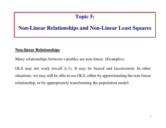
What the linearity assumption does (and does not) mean ◮ first assumption of OLS: linearity. ◮ formally, we say Y is a linear function of the data: ˆ Y i = X i β ◮ parameters/coefficients are linear ◮ we can transform the IVs and DV to improve our model (e.g., remove heteroskedasticity), but parameters must remain linear in order to use OLS ◮ lots of models eschew linearity. An example is the logit model: 1 ˆ Y i = 1 + e − X i β
Acceptable transformations 1 Y = α + β X 2 Y = α + β ( ln ( X )) ln ( Y ) = α + β X ln ( Y ) = α + β ln ( X ) 1 More on this in 407.
Unacceptable transformation Y = ln ( α + β X )
Transforming data ◮ key point: linear transformations change units of measure (e.g., ounces to pounds) but don’t change the distribution. Re-coding is a common example. So if right-skewed data are transformed linearly, the new data will still have right skew. ◮ same goes for relationships between 2+ variables: linear transformations won’t change anything ◮ non-linear transformations will change the distribution. Sometimes we use logs to make linear regression more appropriate. ◮ Example: Jacobson (1990): ...it is clear that linear models of campaign spending are inadequate becase diminishing returns must apply to campaign spending. Green and Krasno recognize this and offer an alternative model which uses log transformations...
Reasons for log transformations 2 ◮ make relationships more linear (Jacobson 1990) ◮ reduce heteroskedasticity or skew ◮ hard sciences do this for certain natural patterns (e.g., exponential processes) ◮ easier interpretation (%s) ◮ key point: transformations change interpretation of coefficients (e.g., in linear-log models, divide coefficient on logged variable by 100) 2 Yanna will talk more about logs.
Outliers Determining whether an outlier is influential: Influence = Leverage*Discrepancy, where leverage is the distance of a given x i from the center of a distribution (mean or centroid) and discrepancy is the distance of Y i from regression line when fitted without observation. In the end, we care about influence = is there one (or two or three) observations that are changing our entire estimated effect?
Quantifying influence 1. DFBETA 2. Cook’s Distance Subjective standard. Most say if either stat is > 1, then problematic.
You’ll need these... library(car) install.packages("nnet") library(nnet) install.packages("MASS") library(MASS) install.packages("stats") library(stats) install.packages("zoo") library(zoo)
DFBETA A measure of how much a coefficient changes with observation included vs. excluded, scaled by the standard error with the observation deleted. From Yanna’s lecture: a<-c(4, 3, 2, 1, 5, 2, 3, 4, 5, 1, 3, 2, 1, 1500) b<-c(1, 0, 1, 1, 0, 1, 0, 1, 0, 1, 0, 0, 1, 1) c<-c(10, 11, 25, 20, 18, 17, 10, 11, 12, 33, 38, 12, 14, 17) plot(a) model<-lm(c ∼ a+b) dfbetasPlots(model) influence.measures(model) dfbetas(model)
dfbetas Plots 0.5 300 0.0 200 a b -0.5 100 -1.0 0 2 4 6 8 12 2 4 6 8 12 Index Index
Cook’s Distance Similar idea as DFBETA. Cook’s Distance quantifies how much coefficient moves within range of possible true values as a result of excluding a given observation. plot(model, which=4, cook.levels=cutoff)
Cook's distance 14 50000 40000 Cook's distance 30000 20000 10000 10 11 0 2 4 6 8 10 12 14 Obs. number lm(c ~ a + b)
Testing for heteroskedasticity Recap: heteroskedasticity is non-constant error variance = loss of efficiency Tests: 1. Breusch-Pagan/Cook-Weisbeg (“BP test”) 2. White’s test
BP Test ◮ we assume that error variances are equal (null), test alternative that they are unequal ◮ idea: regress squared residuals on IVs, see if they predict size of resids ◮ distribution is χ 2 , so critical value depends on degrees of freedom (it will tell you significance) ◮ some simulated heteroskedastic data is on BB if you want to practice ◮ command is easy: library(lmtest) bptest(model)
White’s test ◮ similar idea as BP Test, but instead regresses squared residuals on IVs, squared versions of IVs, and cross-products of regressors ◮ again, distribution is χ 2 , so critical value depends on degrees of freedom (it will tell you significance) ◮ there’s now a package for running White’s test: install.packages("bstats") library(bstats) white.test(model)
Questions?
Recommend


More recommend
Explore More Topics
Stay informed with curated content and fresh updates.