Diagnostics Internally studentized residuals, PRESS residuals or - PowerPoint PPT Presentation

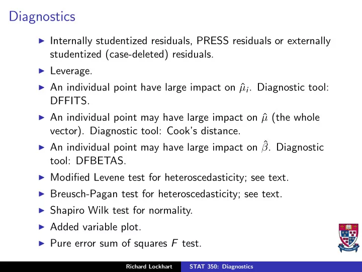
Diagnostics ◮ Internally studentized residuals, PRESS residuals or externally studentized (case-deleted) residuals. ◮ Leverage. ◮ An individual point have large impact on ˆ µ i . Diagnostic tool: DFFITS. ◮ An individual point may have large impact on ˆ µ (the whole vector). Diagnostic tool: Cook’s distance. ◮ An individual point may have large impact on ˆ β . Diagnostic tool: DFBETAS. ◮ Modified Levene test for heteroscedasticity; see text. ◮ Breusch-Pagan test for heteroscedasticity; see text. ◮ Shapiro Wilk test for normality. ◮ Added variable plot. ◮ Pure error sum of squares F test. Richard Lockhart STAT 350: Diagnostics

Leverage ◮ Leverage i is h ii — diagonal entry in hat matrix, H . ◮ Var (ˆ µ i ) = h ii and Var (ˆ ǫ i ) = 1 − h ii so 0 ≤ h ii ≤ 1. ◮ trace ( H ) = p so the h ii average to p / n . ◮ Rule of thumb. h ii > 2 p / n is “large” leverage. ◮ Rule of thumb. h ii > 0 . 5 is large, h ii > 0 . 2 is moderately large. Richard Lockhart STAT 350: Diagnostics

DFFITS Measure change in fitted value for case i after deleting case i : Y i − ˆ ˆ Y i ( i ) ( DFFITS ) i = � MSE ( i ) h ii ◮ Any subscript ( i ) refers to a computation with case i deleted. ◮ Can be computed from externally deleted residual by � multiplying by h ii / (1 − h ii ). Thus can be computed without actually deleting case i and rerunning. ◮ Rule of thumb from text: look out for | DFFITS | > 1 in small � to medium data sets or for | DFFITS | > 2 p / n in large data sets. ◮ But I just examine the few largest values. Richard Lockhart STAT 350: Diagnostics

Cook’s Distance An individual point may have large impact on ˆ µ (the whole vector): j =1 ( ˆ Y j − ˆ � n Y j ( i ) ) 2 D i = p MSE ◮ Can be computed without deleting case from ǫ 2 � � ˆ h ii i D i = p MSE (1 − h ii ) 2 ◮ To judge size compare to F p , n − p , 0 . 90 (lower tail area is 10%, usually found as 1 over upper 10% point of F n − p , p ) and to median ( F p , n − p ). ◮ Bigger than latter is quite serious. ◮ Smaller than former is good. ◮ Between is gray zone. Richard Lockhart STAT 350: Diagnostics

DFBETAS ◮ Intended to measure impact of deleting case i on ˆ β k . ◮ Defined by: β k − ˆ ˆ β k ( i ) DFBETAS k ( i ) = � MSE ( i ) [( X T X ) − 1 ] kk ◮ Same guidelines as DFFITS. ◮ Software not always set up to compute DFBETAS. Richard Lockhart STAT 350: Diagnostics

Tests for Homoscedasticity ◮ Modified Levene test: ◮ Split data set into 2 parts on basis of covariates ◮ Fit regressions in each part separately. ◮ Do 2 sample t -test on mean absolute size of residuals. ◮ Breusch-Pagan test: ◮ Regress squared fitted residual on covariate or covariates ◮ Test for non-zero slope. Richard Lockhart STAT 350: Diagnostics

Tests of Distributional Assumptions ◮ Check assumption of Normality. ◮ Examine Q − Q plot for straightness. ◮ Shapiro-Wilk test applied to residuals ◮ Or correlation test in Q-Q plot. Richard Lockhart STAT 350: Diagnostics

Pure Error Sum of Squares ◮ Sometimes for each (or at least sufficiently many) combination of covariates in a data set, there are several observations. ◮ Can do extra sum of squares F -test to see if our regression model is adequate. ◮ Suppose that x 1 , . . . , x K are the distinct rows of the design matrix ◮ Suppose we have n 1 observations for which the covariate values are those in x 1 , n 2 observations with covariate pattern x 2 and so on. Of course n 1 + · · · + n K = n . ◮ We compare our final fitted model with a so-called saturated model by an extra sum of squares F -test. ◮ To be precise let α 1 be the mean value of Y when the covariate pattern is x 1 , α 2 the mean corresponding to x 2 and so on. ◮ Relabel the n data points as Y i , j ; j = , . . . , n i ; i = 1 , . . . , K ◮ Fit a one way ANOVA model to the Y i , j . Richard Lockhart STAT 350: Diagnostics

Pure Error Sum of Squares ◮ Error sum of squares for this FULL model is K n i � � ( Y i , j − ¯ Y i , · ) 2 ESS FULL = i =1 j =1 ◮ This ESS is called the pure error sum of squares because we have not assumed any particular relation between the mean of Y and the covariate vector x . ◮ We form the F statistic for testing the overall quality of our model by computing the “lack of fit SS” as ESS Restricted − ESS FULL where the restricted model is the final model whose fit we are checking. Richard Lockhart STAT 350: Diagnostics

Example: plaster hardness ◮ 9 different covariate patterns: 3 levels of SAND and 3 levels of FIBRE. ◮ Two ways to compute pure error sum of squares: ◮ Create new variable with 9 levels. ◮ Fit a two way ANOVA with interactions. DATA 0 0 1 61 34 0 0 1 63 16 15 0 2 67 36 15 0 2 69 19 . . . 30 50 9 74 48 Richard Lockhart STAT 350: Diagnostics

SAS CODE data plaster; infile ’plaster1.dat’; input sand fibre combin hardness strength; proc glm data=plaster; model hardness = sand fibre; run; proc glm data=plaster; class sand fibre; model hardness = sand | fibre ; run; proc glm data=plaster; class combin; model hardness = combin; run; Richard Lockhart STAT 350: Diagnostics

EDITED OUTPUT Complete output Sum of Mean Source DF Squares Square F Pr > F Model 2 167.41666667 83.70833333 11.53 0.0009 Error 15 108.86111111 7.25740741 Total 17 276.27777778 Sum of Mean Source DF Squares Square F Pr > F Model 8 202.77777778 25.34722222 3.10 0.0557 Error 9 73.50000000 8.16666667 Total 17 276.27777777 Sum of Mean Source DF Squares Square F Pr > F Model 8 202.77777778 25.34722222 3.10 0.0557 Error 9 73.50000000 8.16666667 Total 17 276.27777778 Richard Lockhart STAT 350: Diagnostics

From the output we can put together a summary ANOVA table Source df SS MS F P Model 2 167.417 83.708 Lack of Fit 6 35.361 5.894 0.722 0.64 Pure Error 9 73.500 8.167 Total (Corrected) 17 276.278 ◮ F statistic is [(108 . 86111111 − 73 . 50000000) / 6] / [8 . 16666667]. ◮ P -value comes from the F 6 , 9 distribution. ◮ P -value not significant: no reason to reject final fitted model which was additive and linear in each of SAND and FIBRE. ◮ Notice that the Error SS are the same for the two-way ANOVA with interactions, which is the second model, and for the 1 way ANOVA. Richard Lockhart STAT 350: Diagnostics

◮ This test is not very powerful in general. ◮ More sensitive tests are available if you know how the model might break down. ◮ For instance, most realistic alternatives will be picked up more easily by checking for quadratic terms in a bivariate polynomial model; see earlier lectures. ◮ Notice that test for any effect of SAND and FIBRE carried out in the one way analysis of variance is not significant. ◮ This is an example of the lack of power found in many F -tests with large numbers of degrees of freedom in the numerator. ◮ If you can guess a reasonable functional form for the effect of the factors (either the additive two way model with no interactions or the even simpler multiple regression model which is the first model above) you will get a more sensitive test usually. Richard Lockhart STAT 350: Diagnostics

Added Variable Plots or partial regression plots ◮ Regress Y on some covariates X 1 . ◮ Get Residuals. ◮ Regress other covariate X 2 on X 1 . ◮ Get Residuals. ◮ Plot two sets of residuals against each other. Richard Lockhart STAT 350: Diagnostics

SENIC data example Fit final selected model: covariates used are STAY, CULTURE, NURSES, NURSE.RATIO. options pagesize=60 linesize=80; data scenic; infile ’scenic.dat’ firstobs=2; input Stay Age Risk Culture Chest Beds School Region Census Nurses Facil; Nratio = Nurses / Census ; proc glm data=scenic; model Risk = Culture Stay Nurses Nratio ; output out=scout P=Fitted PRESS=PRESS H=HAT RSTUDENT=EXTST R=RESID DFFITS=DFFITS COOKD=COOKD; run ; proc print data=scout; Complete SAS Output is here. Richard Lockhart STAT 350: Diagnostics

Index plot of leverages Outlying X Values 4 47 0.30 0.25 0.20 8 Leverage 112 54 0.15 • • • 0.10 • • • • • • • • • • • 0.05 • • • • • • • • • • • • • • • • • • • • • • • • • • • • • • • • • • • • • • • • • • • • • • • • • • • • •• • • • •• • • • • • • • • • • • • • • • • • • • • • • • • • • • • • • • • • • • 0.0 0 20 40 60 80 100 Observation Number Richard Lockhart STAT 350: Diagnostics

Index plot of leverages: discussion ◮ Observations 4, 8, 47, 54 and 112 have leverages over 0.15 ◮ Many more are over 10/113 — the suggested cut off. ◮ I prefer to plot the leverages and look at the largest few. ◮ Observations 4 and 47, in particular, have leverages over 0.3 and should be looked at. ◮ That means scientist thinks about those hospitals! Richard Lockhart STAT 350: Diagnostics