E F s , s t and, after some rearranging, 1 2 ( t s ) 2 . - PowerPoint PPT Presentation
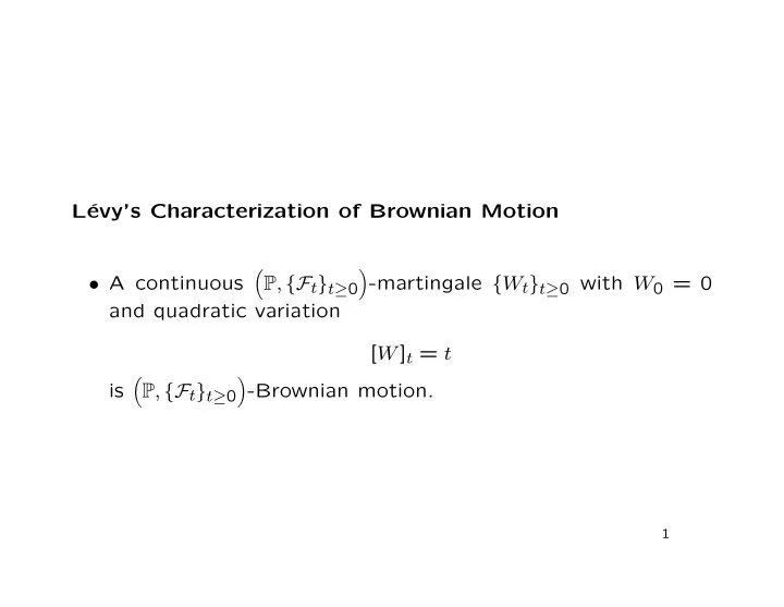
L evys Characterization of Brownian Motion A continuous P , {F t } t 0 -martingale { W t } t 0 with W 0 = 0 and quadratic variation [ W ] t = t is -Brownian motion. P , {F t } t 0 1 Write W t
L´ evy’s Characterization of Brownian Motion � � • A continuous P , {F t } t ≥ 0 -martingale { W t } t ≥ 0 with W 0 = 0 and quadratic variation [ W ] t = t � � is -Brownian motion. P , {F t } t ≥ 0 1
• Write θW t − θ 2 � � △ M ( θ ) = exp 2 t . t • Then by Itˆ o’s formula (generalized!), θW t − θ 2 � � dW t − 1 dt + 1 dM ( θ ) 2 θ 2 M ( θ ) 2 θ 2 M ( θ ) = θ exp 2 t dt t t t θW t − θ 2 � � = θ exp 2 t dW t . • So { M ( θ ) � � } t ≥ 0 is a -martingale. P , {F t } t ≥ 0 t 2
• So for 0 ≤ s < t , � � � M ( θ ) = M ( θ ) � E � F s , s t � and, after some rearranging, 1 2 ( t − s ) θ 2 . � e θ ( W t − W s ) � � � F s = e E � • That is, W t − W s ∼ N (0 , t − s ) and is independent of F s . 3
Stochastic Differential Equation � � • Suppose that { W t } t ≥ 0 is P , {F t } t ≥ 0 -Brownian motion, and Z t = f ( t, W t ). • Then Itˆ o’s formula is f ( t, W t ) + 1 � � 2 f ′′ ( t, W t ) dt + f ′ ( t, W t ) dW t . ˙ dZ t = • If f is invertible, this may be written dZ t = µ ( t, Z t ) dt + σ ( t, Z t ) dW t . 4
• An equation of this form with deterministic functions µ ( t, x ) and σ ( t, x ) is a stochastic differential equation for { Z t } t ≥ 0 . – Note that for given µ ( t, x ) and σ ( t, x ), there may or may not exist a solution; that is, a function f such that Z t = f ( t, W t ); – And if a solution exists, it may or may not be unique. – If µ ( t, x ) and σ ( t, x ) are bounded and uniformly continu- ous in x , a unique solution exists; these conditions are therefore sufficient, but far from necessary. 5
• The quadratic variation of { Z t } t ≥ 0 is � t 0 σ ( s, Z s ) 2 ds. [ Z ] t = • In terms of differentials: d [ Z ] t = σ ( t, Z t ) 2 dt. 6
Integration By Parts • The classical “integration by parts” formula � b � b a f ( x ) g ′ ( x ) dx = [ f ( x ) g ( x )] b a f ′ ( x ) g ( x ) dx a − is a consequence of the rule for the derivative of a product, [ f ( x ) g ( x )] ′ = f ′ ( x ) g ( x ) + f ( x ) g ′ ( x ) . • If f and g are replaced by (semi-)martingales, their covaria- tion must be included. 7
� � • Suppose that { Y t } t ≥ 0 is a P , {F t } t ≥ 0 -semi-martingale: Y t = M ( Y ) + A ( Y ) t t where: – { M ( Y ) � � } t ≥ 0 is a P , {F t } t ≥ 0 -martingale: t – { A ( Y ) } t ≥ 0 is a continuous process of bounded variation. t • Similarly Z t = M ( Z ) + A ( Z ) . t t • Then M ( Y ) , M ( Z ) � � d ( Y t Z t ) = Y t dZ t + Z t dY t + d t . 8
M Y , M Z � � • Here t is the covariation (or mutual variation ) of { M ( Y ) } t ≥ 0 and { M ( Z ) } t ≥ 0 : t t N ( π ) − 1 � � � � M ( Y ) t j +1 − M ( Y ) M ( Z ) t j +1 − M ( Z ) � M ( Y ) , M ( Z ) � � t = lim t j t j δ ( π ) → 0 j =0 where π is a partition of [0 , t ]. • Note that � M ( Y ) , M ( Y ) � � M ( Y ) � t = t ; – that is, the covariation of a process with itself is just its quadratic variation. 9
• For example, if dY t = µ ( t, Y t ) dt + σ ( t, Y t ) dW t and dZ t = ˜ µ ( t, Z t ) dt + ˜ σ ( t, Z t ) dW t and { M ( Y ) } t ≥ 0 and { M ( Z ) � � } t ≥ 0 are the P , {F t } t ≥ 0 -martingales t t � t M ( Y ) = 0 σ ( s, Y s ) dW s , t � t M ( Z ) = 0 ˜ σ ( s, Z s ) dW s , t then � t M ( Y ) , M ( Z ) � � t = 0 σ ( s, Y s )˜ σ ( s, Z s ) ds. 10
• In that example, { Y t } t ≥ 0 and { Z t } t ≥ 0 are driven by the same Brownian motion { W t } t ≥ 0 . • More generally, if instead σ ( t, Z t ) d ˜ dZ t = ˜ µ ( t, Z t ) dt + ˜ W t and { M ( Z ) } t ≥ 0 is the martingale t � t M ( Z ) σ ( s, Z s ) d ˜ = 0 ˜ W s , t where W t and ˜ W t have correlation ρ , then � t M ( Y ) , M ( Z ) � � t = 0 σ ( s, Y s )˜ σ ( s, Z s ) ρds. 11
Stochastic Fubini Theorem • Interchanging a stochastic and a non-stochastic integral. � � • Let Ω , F , {F t } t ≥ 0 , P be a filtered probability space, and let � � { M t } t ≥ 0 be a continuous P , {F t } t ≥ 0 -martingale with M 0 = 0. Suppose that Φ( t, r, ω ) : R + × R + × Ω �→ R is a bounded {F t } t ≥ 0 -predictable random variable. Then for each fixed T > 0, � t � t � � R Φ( s, r, ω ) 1 [0 ,T ] ( r ) drdM s = 0 Φ( s, r, ω ) 1 [0 ,T ] ( r ) dM s dr. 0 R • In a more familiar notation, � t � T � T � t 0 Φ s ( r ) drdM s = 0 Φ s ( r ) dM s dr. 0 0 12
Recommend
More recommend
Explore More Topics
Stay informed with curated content and fresh updates.
