Multivariate fractional Brownian motion Fr ed eric Lavancier - PowerPoint PPT Presentation
Self-similarity Integral representations Covariance Increments Existence of the covariance Identification Some applications Multivariate fractional Brownian motion Fr ed eric Lavancier Laboratoire de Math ematiques Jean Leray
Self-similarity Integral representations Covariance Increments Existence of the covariance Identification Some applications Multivariate fractional Brownian motion Fr´ ed´ eric Lavancier Laboratoire de Math´ ematiques Jean Leray Universit´ e de Nantes Joint works with P.-O. Amblard, J.-F. Coeurjolly, A. Philippe and D. Surgailis.
Self-similarity Integral representations Covariance Increments Existence of the covariance Identification Some applications Axiomatic definition Definition A multivariate fractional Brownian motion (mfBm) with parameter H ∈ (0 , 1) p is a p-multivariate process satisfying the three following properties Gaussianity Self similarity with parameter H = ( H 1 , . . . , H p ) ∈ (0 , 1) p � � fidi λ H 1 X 1 ( t ) , · · · , λ H p X p ( t ) ( X 1 ( λ t ) , · · · , X p ( λ t )) t ∈ R = ∀ λ > 0 t ∈ R Stationarity of the increments → This is a particular case of operator self-similar processes: fidi = t H X ( t ) for some matrix H [Laha, Rohagi’81 ; Hudson, Mason’82] , X ( λ t ) by taking H = diag ( H 1 , . . . , H p ). → Each component ( X j ( t )) t ∈ R is a fractional Brownian motion. → Motivation : study of correlated fractional Brownian motions
Self-similarity Integral representations Covariance Increments Existence of the covariance Identification Some applications Axiomatic definition Definition A multivariate fractional Brownian motion (mfBm) with parameter H ∈ (0 , 1) p is a p-multivariate process satisfying the three following properties Gaussianity Self similarity with parameter H = ( H 1 , . . . , H p ) ∈ (0 , 1) p � � fidi λ H 1 X 1 ( t ) , · · · , λ H p X p ( t ) ( X 1 ( λ t ) , · · · , X p ( λ t )) t ∈ R = ∀ λ > 0 t ∈ R Stationarity of the increments → This is a particular case of operator self-similar processes: fidi = t H X ( t ) for some matrix H [Laha, Rohagi’81 ; Hudson, Mason’82] , X ( λ t ) by taking H = diag ( H 1 , . . . , H p ). → Each component ( X j ( t )) t ∈ R is a fractional Brownian motion. → Motivation : study of correlated fractional Brownian motions
Self-similarity Integral representations Covariance Increments Existence of the covariance Identification Some applications Some examples : Below, the correlation between all couples of FBM’s is 0 . 6 H ∈ [0 . 3 , 0 . 4] H ∈ [0 . 8 , 0 . 9] H ∈ [0 . 4 , 0 . 8] (decentered)
Self-similarity Integral representations Covariance Increments Existence of the covariance Identification Some applications Justification of joint self-similarity 1 Integral representations 2 Covariance structure of the mfBm 3 The increment process 4 Existence of the covariance function 5 Identification 6 Some applications 7
Self-similarity Integral representations Covariance Increments Existence of the covariance Identification Some applications Justification of joint self-similarity As for the univariate case, we have the following Lamperti results: Theorem (Lamperti’62; Hudson, Mason’82) Stationarity ↔ Self-similarity. 1 ( Y ( t )) t ∈ R is a p-multivariate stationary process if and only if there exists H ∈ (0 , 1) p such that ( t H 1 Y 1 (log( t )) , . . . , t H p Y p (log( t ))) t ∈ R is a p-multivariate self-similar process. Self-similarity in limiting processes. 2 Let ( X ( t )) t ∈ R be a p-multivariate proper process, continuous in probability. If there exist a p-multivariate process ( Y ( t )) t ∈ R and p real functions a 1 , ...., a p such that n →∞ ( a 1 ( n ) Y 1 ( nt ) , . . . , a p ( n ) Y p ( nt )) − − − → X ( t ) , fidi then the multivariate process ( X ( t )) is self-similar. Conversely, any multivariate self-similar process can be obtained as a such limit.
Self-similarity Integral representations Covariance Increments Existence of the covariance Identification Some applications Justification of joint self-similarity As for the univariate case, we have the following Lamperti results: Theorem (Lamperti’62; Hudson, Mason’82) Stationarity ↔ Self-similarity. 1 ( Y ( t )) t ∈ R is a p-multivariate stationary process if and only if there exists H ∈ (0 , 1) p such that ( t H 1 Y 1 (log( t )) , . . . , t H p Y p (log( t ))) t ∈ R is a p-multivariate self-similar process. Self-similarity in limiting processes. 2 Let ( X ( t )) t ∈ R be a p-multivariate proper process, continuous in probability. If there exist a p-multivariate process ( Y ( t )) t ∈ R and p real functions a 1 , ...., a p such that n →∞ ( a 1 ( n ) Y 1 ( nt ) , . . . , a p ( n ) Y p ( nt )) − − − → X ( t ) , fidi then the multivariate process ( X ( t )) is self-similar. Conversely, any multivariate self-similar process can be obtained as a such limit.
Self-similarity Integral representations Covariance Increments Existence of the covariance Identification Some applications An example: partial sums of superlinear processes Let ( ε j ( k )) k ∈ Z , j = 1 , . . . , p be p independent i.i.d. sequences with zero mean and unit variance. Let us consider the superlinear processes p � � Z i ( t ) = ψ i , j ( t − k ) ε j ( k ) , i = 1 , . . . , p , j =1 k ∈ Z where � k ∈ Z ψ 2 i , j ( k ) < ∞ . Assume that ψ i , j ( k ) = ψ + i , j ( k ) + ψ − i , j ( k ) where ψ + i , j ( k ) satisfies one of the following conditions: d + i , j − 1 � � (i) ψ + α + as | k | → ∞ , with 0 < d + i , j < 1 2 and α + i , j ( k ) = i , j + o (1) k i , j � = 0, + d + i , j − 1 � � (ii) ψ + α + 2 < d + k ∈ Z ψ + as | k | → ∞ , with − 1 i , j ( k ) = i , j + o (1) k i , j < 0, � i , j ( k ) = 0 and + α + i , j � = 0, � � � ψ + � < ∞ and let α + k ∈ Z ψ + i , j ( k ) � = 0, d + (iii) � i , j := � i , j ( k ) i , j := 0. � � k ∈ Z ψ − i , j ( k ) is assumed to satisfy ( i ), ( ii ) or ( iii ) with k − , d − i , j and α − i , j .
Self-similarity Integral representations Covariance Increments Existence of the covariance Identification Some applications An example: partial sums of superlinear processes Proposition Let d i = max ( d + i 1 , d − i 1 , · · · , d + ip , d − ip ) , for i = 1 , . . . , p. Consider the vector of partial sums, for τ ∈ R , [ n τ ] [ n τ ] � � n − d 1 − (1 / 2) Z 1 ( t ) , · · · , n − d p − (1 / 2) . S n ( τ ) = Z p ( t ) t =1 t =1 Then the finite dimensional distributions of ( S n ( τ )) τ ∈ R converges in law towards a p-mfBm ( X ( τ )) τ ∈ R with Hurst exponent ( d 1 + 1 / 2 , . . . , d p + 1 / 2) . Conversely any p-mfBm with Hurst exponent ( H 1 , . . . , H p ) with ∀ i H i � = 1 / 2 can be obtained as such a limit.
Self-similarity Integral representations Covariance Increments Existence of the covariance Identification Some applications Proof. Cramer-Wold device + convergence of discrete stochastic integral [Surgailis’82]. Idea of the latter (univariate case): If Z ( t ) = � n k ∈ Z ψ ( t − k ) ε ( k ), then n n n � � � n − d − 1 / 2 Z ( t ) = n − d − 1 / 2 ψ ( t − k ) ε ( k ) t =1 t =1 k ∈ Z n � � n − d ψ ( t − k ) n − 1 / 2 ε ( k ) = k ∈ Z t =1 �� k n n ; k + 1 �� � � n − d = ψ ( t − k ) W n n t =1 k ∈ Z where for any interval I , W n ( I ) = n − 1 / 2 � j ∈ nI ε ( j ). � ( k +1) / n n n � n − d − 1 / 2 � � � n − d Z ( t ) = ψ ( t − k ) W n ( dx ) = f n ( x ) W n ( dx ) k / n t =1 t =1 k ∈ Z where f n ( x ) = n − d � n t =1 ψ ( t − ⌊ nx ⌋ ). Lemma (Surgailis’82) L 2 f n ( x ) W n ( dx ) L � � If f n → f then → f ( x ) W ( dx ) where W is a Gaussian white noise. So the proof reduces to study the L 2 convergence of f n ... provided we have an integral representation for the mfBm.
Self-similarity Integral representations Covariance Increments Existence of the covariance Identification Some applications Proof. Cramer-Wold device + convergence of discrete stochastic integral [Surgailis’82]. Idea of the latter (univariate case): If Z ( t ) = � n k ∈ Z ψ ( t − k ) ε ( k ), then n n n � � � n − d − 1 / 2 Z ( t ) = n − d − 1 / 2 ψ ( t − k ) ε ( k ) t =1 t =1 k ∈ Z n � � n − d ψ ( t − k ) n − 1 / 2 ε ( k ) = k ∈ Z t =1 �� k n n ; k + 1 �� � � n − d = ψ ( t − k ) W n n t =1 k ∈ Z where for any interval I , W n ( I ) = n − 1 / 2 � j ∈ nI ε ( j ). � ( k +1) / n n n � n − d − 1 / 2 � � � n − d Z ( t ) = ψ ( t − k ) W n ( dx ) = f n ( x ) W n ( dx ) k / n t =1 t =1 k ∈ Z where f n ( x ) = n − d � n t =1 ψ ( t − ⌊ nx ⌋ ). Lemma (Surgailis’82) L 2 f n ( x ) W n ( dx ) L � � If f n → f then → f ( x ) W ( dx ) where W is a Gaussian white noise. So the proof reduces to study the L 2 convergence of f n ... provided we have an integral representation for the mfBm.
Recommend
More recommend
Explore More Topics
Stay informed with curated content and fresh updates.
