Inference for periodic Ornstein Uhlenbeck process driven by - PowerPoint PPT Presentation

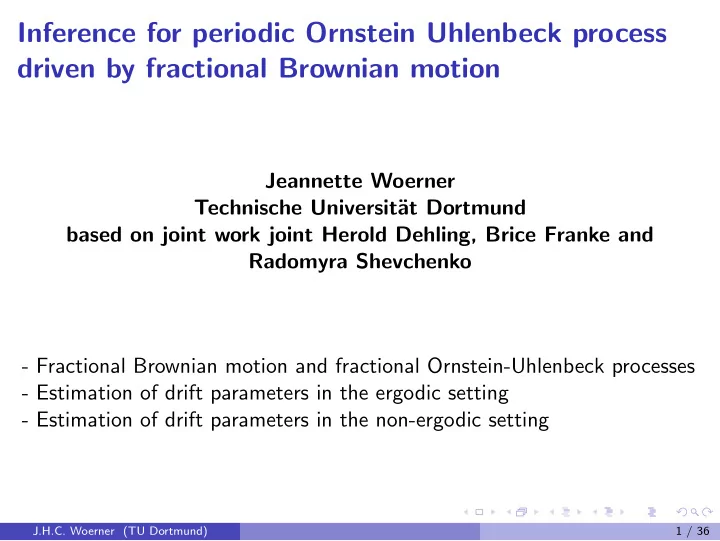
Inference for periodic Ornstein Uhlenbeck process driven by fractional Brownian motion Jeannette Woerner Technische Universit¨ at Dortmund based on joint work joint Herold Dehling, Brice Franke and Radomyra Shevchenko - Fractional Brownian motion and fractional Ornstein-Uhlenbeck processes - Estimation of drift parameters in the ergodic setting - Estimation of drift parameters in the non-ergodic setting FoGruLogo s mall tud l ogo c myk . pdf J.H.C. Woerner (TU Dortmund) 1 / 36

Motivation Empirical evidence in data: - often mean-reverting property or in other cases explosive behaviour - specific correlation structure, e.g. long range dependence - often saisonalities are present Questions: - How can we model this features? - How can we infer involved quantities? FoGruLogo s mall tud l ogo c myk . pdf J.H.C. Woerner (TU Dortmund) 2 / 36

Fractional Brownian Motion A fractional Brownian motion (fBm) with Hurst parameter H ∈ (0 , 1), B H = { B H t , t ≥ 0 } is a zero mean Gaussian process with the covariance function s ) = 1 2( t 2 H + s 2 H − | t − s | 2 H ) , E ( B H t B H s , t ≥ 0 . Properties: - Correlation For H ∈ ( 1 2 , 1) the process possesses long memory and for H ∈ (0 , 1 2 ) the behaviour is chaotic . 2 , B H coincides with the classical Brownian motion. - For H = 1 - H¨ older continuous paths of the order γ < H . - Gaussian increments - Selfsimilarity: { a − H B H at , t ≥ 0 } and { B H t , t ≥ 0 } have the same distribution. FoGruLogo s mall tud l ogo c myk . pdf - if H � = 0 . 5 not a semimartingale . J.H.C. Woerner (TU Dortmund) 3 / 36

FoGruLogo s mall tud l ogo c myk . pdf J.H.C. Woerner (TU Dortmund) 4 / 36

Implications of this properties - fractional Brownian motion is non-Markovian : usual martingale approaches do not work, - increments are not independent, we cannot use classical limit theorems for independent random variables, - Itˆ o integration does not work, we need a different type of integration, the easiest is a pathswise Riemann-Stieltjes integral . Other possibility is a divergence integral which allows for a generalization of the Itˆ o formula. FoGruLogo s mall tud l ogo c myk . pdf J.H.C. Woerner (TU Dortmund) 5 / 36

Ornstein-Uhlenbeck Process A classical Ornstein-Uhlenbeck process is given by the stochastic differential equation dX t = − λ X t dt + dW t where W denotes a Brownian motion. It possesses the solution � t X t = X 0 e − λ t + e − λ ( t − s ) dW s 0 and for λ > 0 it is mean-reverting and ergodic , for λ < 0 it is non-ergodic . Popular generalizations are to replace the Brownian motion by a L´ evy process or a fractional Brownian motion. FoGruLogo s mall tud l ogo c myk . pdf J.H.C. Woerner (TU Dortmund) 6 / 36

Perodic fractional Ornstein-Uhlenbeck processes We consider the stochastic process ( X t ) given by the stochastic differential equation dX t = ( L ( t ) − α X t ) dt + σ dB H t , with X 0 = ξ 0 , where ξ 0 is square integrable, independent of the fractional Brownian motion ( B H t ) t ∈ R . We have a period drift function L ( t ) = � p i =1 µ i φ i ( t ), where φ i ( t ); i = 1 , ..., p are bounded and periodic with the same period ν . µ i ; i = 1 , ..., p are unknown parameters as well as α . But we know if it is positive or negative, furthermore σ , H ∈ (1 / 2 , 3 / 4) and p are known. We assume that the functions φ i ; i = 1 , ..., p are orthonormal in L 2 ([0 , ν ] , ν − 1 ℓ ) and that φ i ; i = 1 , ..., p are bounded by a constant C > 0. We observe the process continuously up to time T = n ν and let n → ∞ . FoGruLogo s mall tud l ogo c myk . pdf J.H.C. Woerner (TU Dortmund) 7 / 36

Related work Belfadli, Es-Sebaiy and Ouknine (2011): Parameter estimation for fractional Ornstein Uhlenbeck processes: non-ergodic case Dehling, Franke and Kott (2010): Estimation in periodic Ornstein-Uhlenbeck processes Kleptsyna and Le Breton (2002): MLE for a fractional Ornstein-Uhlenbeck process based on associated semimartingales Hu and Nualart (2010): Least-squares estimator for a fractional Ornstein-Uhlenbeck process. FoGruLogo s mall tud l ogo c myk . pdf J.H.C. Woerner (TU Dortmund) 8 / 36

Some analytic background For a fixed [0 , T ] the space H is defined as the closure of the set of real valued step functions on [0 , T ] with respect to the scalar product < 1 [0 , t ] , 1 [0 , s ] > H = E ( B H t B H s ). The mapping 1 [0 , t ] → B H t can be extended to an isometry between H and the Gaussian space associated with B H . Noting that � t � s | u − v | 2 H − 2 dudv E ( B H t B H s ) = H (2 H − 1) 0 0 we obtain the useful isometry properties � t � t � t φ ( s ) dB H s ) 2 ) = H (2 H − 1) φ ( u ) φ ( v ) | u − v | 2 H − 2 dudv E (( 0 0 0 � t � t � s φ ( s ) dB H φ ( u ) dB H u dB H E ( s ) = 0 . FoGruLogo s mall s 0 0 0 tud l ogo c myk . pdf J.H.C. Woerner (TU Dortmund) 9 / 36

Divergence integral � t 0 u s dB H For the ergodic case, we have to interpret the integrals s as divergence integral , i.e. � t u s dB H s = δ ( u 1 [0 , s ] ) 0 or � t � t � t � s D r u s | s − r | 2 H − 2 drds u s dB H u s ∂ B H s = s + H (2 H − 1) 0 0 0 0 If we used a straight forward Riemann Stieltjes integral , it has been shown in Hu and Nualart (2010) that already the simple case of estimating � n ν X t dX t α in a non-periodic setting by ˆ α = − t dt would not lead to a 0 � n ν X 2 0 consistent estimator. Namely in the framework of Riemann Stieltjes X 2 α simplifies to − t dt , which tends to zero as n → ∞ . integrals ˆ n ν � n ν X 2 FoGruLogo s mall 2 0 tud l ogo c myk . pdf J.H.C. Woerner (TU Dortmund) 10 / 36

Some preliminary facts on the model: case α > 0 ( X t ) t ≥ 0 given by � t � t � � X t = e − α t e α s L ( s ) ds + σ e α s dB H ξ 0 + ; t ≥ 0 s 0 0 is the unique almost surely continuous solution of equation dX t = ( L ( t ) − α X t ) dt + σ dB H t with initial condition X 0 = ξ 0 . In the following we need a stationary solution. ( ˜ X t ) t ≥ 0 given by �� t � t � ˜ X t := e − α t e α s L ( s ) ds + σ e α s dB H s −∞ −∞ is an almost surely continuous stationary solution of the equation above. FoGruLogo s mall Note that for large t the difference between the two representations tends tud l ogo c myk . pdf to zero. J.H.C. Woerner (TU Dortmund) 11 / 36

Construction of a stationary and ergodic sequence For the limit theorems implying consistency and asymptotic normality we need a stationary and ergodic sequence . Assume that L is periodic with period ν = 1, then the sequence of C [0 , 1]-valued random variables W k ( s ) := ˜ X k − 1+ s , 0 ≤ s ≤ 1 , k ∈ N is stationary and ergodic . FoGruLogo s mall tud l ogo c myk . pdf J.H.C. Woerner (TU Dortmund) 12 / 36

Proof. Since L is periodic, the function � t ˜ h ( t ) := e − α t e α s L ( s ) ds −∞ is also periodic on R . We have for any t ∈ [0 , 1] that � t � 1 0 W k ( t ) = ˜ h ( t )+ σ e − α t e α s dB H � e − α ( t +1 − j ) e α s dB H s + k − 1 + σ s + j + k − 2 . 0 0 j = −∞ FoGruLogo s mall tud l ogo c myk . pdf J.H.C. Woerner (TU Dortmund) 13 / 36

Thus, we have the almost sure representation 0 W k ( · ) = ˜ � e α ( j − 1) F ( Y j + k − 1 ) h ( · ) + F 0 ( Y k ) + j = −∞ with the functionals � t � � t �→ σ e − α t e α s d ω ( s ) F 0 : C [0 , 1] → C [0 , 1]; ω �→ , 0 � 1 F : C [0 , 1] → C [0 , 1]; ω �→ σ e − α t e α s d ω ( s ) 0 and the C [0 , 1]-valued random variable � s �→ B H s + l − 1 − B H � l − 1 ; 0 ≤ s ≤ 1 Y l := . Since ( Y l ) is defined via the increments of fractional Brownian motion, they form a sequence of Gaussian random variables which is stationary and ergodic . This implies that the sequence of ( W k ) k ∈ N is stationary and ergodic. FoGruLogo s mall tud l ogo c myk . pdf J.H.C. Woerner (TU Dortmund) 14 / 36

Motivation of the estimator We start with the more general problem of a p + 1-dimensional parameter vector θ = ( θ 1 , ..., θ p +1 ) in the stochastic differential equation dX t = θ f ( t , X t ) dt + σ dB H t , where f ( t , x ) = ( f 1 ( t , x ) , ..., f p +1 ( t , x )) t with suitable real valued functions f i ( t , x ); 1 ≤ i ≤ p . A discretization of the above equation on the time interval [0 , T ] yields for ∆ t := T / N and i = 1 , ..., N p +1 � � � B H ( i +1)∆ t − B H X ( i +1)∆ t − X i ∆ t = f j ( i ∆ t , X i ∆ t ) θ j ∆ t + σ . i ∆ t j =1 Now we can use a least-squares approach and minimize 2   N p +1 � � G : ( θ 1 , ..., θ p +1 ) �→  X ( i +1)∆ t − X i ∆ t − f j ( i ∆ t , X i ∆ t ) θ j ∆ t .  FoGruLogo s mall i =1 j =1 tud l ogo c myk . pdf J.H.C. Woerner (TU Dortmund) 15 / 36

Least-squares estimator for general setting As in Franke and Kott (2013) in a L´ evy setting a least-squares estimator may be deduces which motivates the continuous time estimator θ T = Q − 1 ˆ T P T with � T � T   0 f 1 ( t , X t ) f 1 ( t , X t ) dt . . . 0 f 1 ( t , X t ) f p +1 ( t , X t ) dt . . . . Q T =   . .   � T � T 0 f p +1 ( t , X t ) f 1 ( t , X t ) dt . . . 0 f p +1 ( t , X t ) f p +1 ( t , X t ) dt and �� T � T � t P T := f 1 ( t , X t ) dX t , ..., f p ( t , X t ) dX t . 0 0 FoGruLogo s mall tud l ogo c myk . pdf J.H.C. Woerner (TU Dortmund) 16 / 36