Interpolation, Growth Conditions, and Stochastic Gradient Descent - PowerPoint PPT Presentation
Interpolation, Growth Conditions, and Stochastic Gradient Descent Aaron Mishkin, amishkin@cs.ubc.ca 1 45 Training neural networks is dangerous work! 2 45 Chapter 1: Introduction 3 45 Chapter 1: Goal Premise : modern neural networks
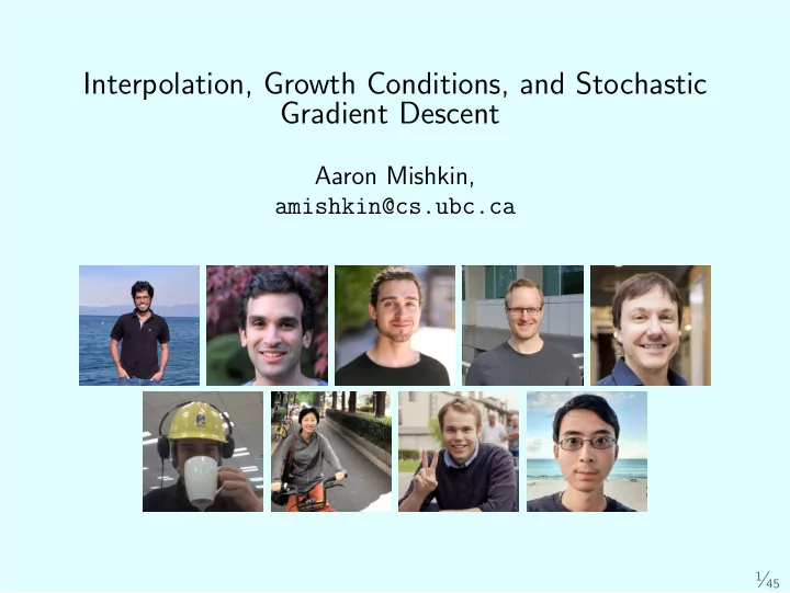
Interpolation, Growth Conditions, and Stochastic Gradient Descent Aaron Mishkin, amishkin@cs.ubc.ca 1 ⁄ 45
Training neural networks is dangerous work! 2 ⁄ 45
Chapter 1: Introduction 3 ⁄ 45
Chapter 1: Goal Premise : modern neural networks are extremely flexible and can exactly fit many training datasets. • e.g. ResNet-34 on CIFAR-10. Question : what is the complexity of learning these models using stochastic gradient descent (SGD)? 4 ⁄ 45
Chapter 1: Model Fitting in ML https://towardsdatascience.com/challenges-deploying-machine-learning-models-to-production-ded3f9009cb3 5 ⁄ 45
Chapter 1: Stochastic Gradient Descent “Stochastic gradient descent (SGD) is today one of the main workhorses for solving large-scale supervised learning and optimization problems.” —Drori and Shamir [2019] 6 ⁄ 45
Chapter 1: Consensus Says. . . . . . and also Agarwal et al. [2017], Assran and Rabbat [2020], Assran et al. [2018], Bernstein et al. [2018], Damaskinos et al. [2019], Geffner and Domke [2019], Gower et al. [2019], Grosse and Salakhudinov [2015], Hofmann et al. [2015], Kawaguchi and Lu [2020], Li et al. [2019], Patterson and Gibson [2017], Pillaud-Vivien et al. [2018], Xu et al. [2017], Zhang et al. [2016] 7 ⁄ 45
Chapter 1: Challenges in Optimization for ML Stochastic gradient methods are the most popular algorithms for fitting ML models, SGD: w k +1 = w k − η k ∇ f i ( w k ) . But practitioners face major challenges with • Speed : step-size/averaging controls convergence rate. • Stability : hyper-parameters must be tuned carefully. • Generalization : optimizers encode statistical tradeoffs. 8 ⁄ 45
Chapter 1: Challenges in Optimization for ML Stochastic gradient methods are the most popular algorithms for fitting ML models, SGD: w k +1 = w k − η k ∇ f i ( w k ) . But practitioners face major challenges with • Speed : step-size/averaging controls convergence rate. • Stability : hyper-parameters must be tuned carefully. • Generalization : optimizers encode statistical tradeoffs. 9 ⁄ 45
Chapter 1: Better Optimization via Better Models Idea : exploit “over-parameterization” for better optimization. • Intuitively, gradient noise goes to 0 if all data are fit exactly. • No need for decreasing step-sizes, or averaging for convergence. 10 ⁄ 45
Chapter 2: Interpolation and Growth Conditions 11 ⁄ 45
Chapter 2: Assumptions We need assumptions to analyze the complexity of SGD. Goal : Minimize f : R d → R , where • f is lower-bounded : ∃ w ∗ ∈ R d such that ∀ w ∈ R d , f ( w ∗ ) ≤ f ( w ) • f is L- smooth : w �→ ∇ f ( w ) is L -Lipschitz, ∀ w, u ∈ R d , �∇ f ( w ) − ∇ f ( u ) � 2 ≤ L � w − u � 2 • (Optional) f is µ - strongly-convex : ∃ µ ≥ 0 such that, f ( u ) ≥ f ( w ) + �∇ f ( w ) , u − w � + µ 2 � u − w � 2 ∀ w, u ∈ R d . 2 12 ⁄ 45
Chapter 2: Stochastic First-Order Oracles Stochastic Oracles : 1. At each iteration k , query oracle O for stochastic estimates f ( w k , z k ) and ∇ f ( w k , z k ) . 2. f ( w k , · ) is a deterministic function of random variable z k . 3. O is unbiased , meaning E z k [ f ( w k , z k )] = f ( w k ) and E z k [ ∇ f ( w k , z k )] = ∇ f ( w k ) . 4. O is individually-smooth , meaning f ( · , z k ) is L max -smooth, ∀ w, u ∈ R d , �∇ f ( w, z k ) − ∇ f ( u, z k ) � 2 ≤ L max � w − u � 2 almost surely. 13 ⁄ 45
Chapter 2: Defining Interpolation Definition (Interpolation: Minimizers) ( f, O ) satisfies minimizer interpolation if f ( w ) w ′ ∈ arg min f = ⇒ w ′ ∈ arg min f ( · , z k ) a.s. w ∗ f ( w, z ) Definition (Interpolation: Stationary Points) ( f, O ) satisfies stationary-point interpolation if w ′ a.s. ∇ f ( w ′ ) = 0 = ⇒ ∇ f ( w ′ , z k ) = 0 . w ′ w ∗ Definition (Interpolation: Mixed) ( f, O ) satisfies mixed interpolation if w ′ ∈ arg min f = a.s. ⇒ ∇ f ( w ′ , z k ) = 0 . w ∗ 14 ⁄ 45
Chapter 2: Interpolation Relationships • All three definitions occur in the literature without distinction! • We formally define them and characterize their relationships. 15 ⁄ 45
Chapter 2: Interpolation Relationships • All three definitions occur in the literature without distinction! • We formally define them and characterize their relationships. Lemma (Interpolation Relationships) Let ( f, O ) be arbitrary. Then only the following relationships hold: Minimizer Interpolation = ⇒ Mixed Interpolation and Stationary-Point Interpolation = ⇒ Mixed Interpolation . However, if f and f ( · , z k ) are invex (almost surely) for all k , then the three definitions are equivalent. Note: invexity is weaker than convexity and implied by it. 15 ⁄ 45
Chapter 2: Using Interpolation There are two obvious ways that we can leverage interpolation: 1. Relate interpolation to global behavior of O . ◮ This was first done using the weak and strong growth conditions by Vaswani et al. [2019a]. 2. Use interpolation in a direct analysis of SGD. ◮ This was first done by Bassily et al. [2018], who analyzed SGD under a curvature condition. We do both, starting with weak/strong growth. 16 ⁄ 45
Growth Conditions: Well-behaved Oracles There are many possible regularity assumptions on O . � �∇ f ( w, z k ) � 2 � ≤ σ 2 , Bounded Gradients : E • Proposed by Robbins and Monro in their analysis of SGD. 17 ⁄ 45
Growth Conditions: Well-behaved Oracles There are many possible regularity assumptions on O . � �∇ f ( w, z k ) � 2 � ≤ σ 2 , Bounded Gradients : E • Proposed by Robbins and Monro in their analysis of SGD. � �∇ f ( w, z k ) � 2 � ≤ �∇ f ( w ) � 2 + σ 2 , Bounded Variance : E • Commonly used in the stochastic approximation setting. 17 ⁄ 45
Growth Conditions: Well-behaved Oracles There are many possible regularity assumptions on O . � �∇ f ( w, z k ) � 2 � ≤ σ 2 , Bounded Gradients : E • Proposed by Robbins and Monro in their analysis of SGD. � �∇ f ( w, z k ) � 2 � ≤ �∇ f ( w ) � 2 + σ 2 , Bounded Variance : E • Commonly used in the stochastic approximation setting. � �∇ f ( w, z k ) � 2 � ≤ ρ �∇ f ( w ) � 2 + σ 2 . Strong Growth+Noise : E • Satisfied when O is individually-smooth and bounded below. 17 ⁄ 45
Growth Conditions: Strong and Weak Growth We obtain the strong and weak growth conditions as follows: ≤ ρ �∇ f ( w ) � 2 + σ 2 . � �∇ f ( w, z k ) � 2 � Strong Growth+Noise : E • Does not imply interpolation. 18 ⁄ 45
Growth Conditions: Strong and Weak Growth We obtain the strong and weak growth conditions as follows: ≤ ρ �∇ f ( w ) � 2 + σ 2 . � �∇ f ( w, z k ) � 2 � Strong Growth+Noise : E • Does not imply interpolation. � �∇ f ( w, z k ) � 2 � ≤ ρ �∇ f ( w ) � 2 . Strong Growth : E • Implies stationary-point interpolation. 18 ⁄ 45
Growth Conditions: Strong and Weak Growth We obtain the strong and weak growth conditions as follows: ≤ ρ �∇ f ( w ) � 2 + σ 2 . � �∇ f ( w, z k ) � 2 � Strong Growth+Noise : E • Does not imply interpolation. � �∇ f ( w, z k ) � 2 � ≤ ρ �∇ f ( w ) � 2 . Strong Growth : E • Implies stationary-point interpolation. � �∇ f ( w, z k ) � 2 � ≤ α ( f ( w ) − f ( w ∗ )) . Weak Growth : E • Implies mixed interpolation. 18 ⁄ 45
Growth Conditions: Interpolation + Smoothness Lemma (Interpolation and Weak Growth) Assume f is L -smooth and O is L max individually- smooth. If minimizer interpolation holds, then weak growth also holds with α ≤ L max L . Lemma (Interpolation and Strong Growth) Assume f is L -smooth and µ strongly-convex and O is L max individually-smooth. If minimizer interpolation holds, then strong growth also holds with ρ ≤ L max µ . Comments : • This improve on the original result by Vaswani et al. [2019a], which required convexity. • Oracle framework extends relationship beyond finite-sums. • See thesis for additional results on weak/strong growth. 19 ⁄ 45
Chapter 3: Stochastic Gradient Descent 20 ⁄ 45
Chapter 3: Fixed Step-size SGD Fixed Step-Size SGD 0. Choose an initial point w 0 ∈ R d . 1. For each iteration k ≥ 0 : 1.1 Query O for ∇ f ( w k , z k ) . 1.2 Update input as w k +1 = w k − η ∇ f ( w k , z k ) . 21 ⁄ 45
Chapter 3: Fixed Step-size SGD Prior work for SGD under growth conditions or interpolation: • Convergence under strong growth [Cevher and Vu, 2019, Schmidt and Le Roux, 2013]. • Convergence under weak growth [Vaswani et al., 2019a]. • Convergence under interpolation [Bassily et al., 2018]. 22 ⁄ 45
Chapter 3: Fixed Step-size SGD Prior work for SGD under growth conditions or interpolation: • Convergence under strong growth [Cevher and Vu, 2019, Schmidt and Le Roux, 2013]. • Convergence under weak growth [Vaswani et al., 2019a]. • Convergence under interpolation [Bassily et al., 2018]. We still provide many new and improved results! • Bigger step-sizes and faster rates for convex and strongly-convex objectives. • Almost-sure convergence under weak/strong growth. • Trade-offs between growth conditions and interpolation. 22 ⁄ 45
Chapter 4: Line Search 23 ⁄ 45
Recommend
More recommend
Explore More Topics
Stay informed with curated content and fresh updates.
