Gradient Analysis NMDS Indirect Gradient Analysis NMDS Direct - PowerPoint PPT Presentation
Multivariate Fundamentals: Rotation/Distance Gradient Analysis NMDS Indirect Gradient Analysis NMDS Direct Gradient Analysis Objective: Use one dataset to explain another Use the spatial patterns of each dataset to try and understand the
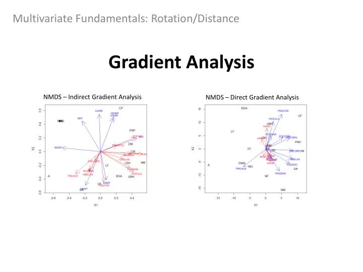
Multivariate Fundamentals: Rotation/Distance Gradient Analysis NMDS – Indirect Gradient Analysis NMDS – Direct Gradient Analysis
Objective: Use one dataset to explain another Use the spatial patterns of each dataset to try and understand the structure and data variation in terms of gradients in space of variables on multiple levels E.g. environmental factors, species populations and characteristics of communities “Gradient Analysis” is an umbrella term which includes both rotation -based and distance-based techniques All of which are aiming to determine “What in dataset A explains dataset B”?
Gradient analysis Data gets separated into 2 distinct datasets that have a spatial link: Predictor Variables Response Variables MAT MAP AHI … Sp1 Sp2 Sp3 … Which set of variables is classified as the response vs the predictors is not always clear You have to use some logic to say what set of variables potentially influences another
Direct gradient analysis Ordinates the data according to the independent variable (e.g. climate) and then investigates how the dependent variables (e.g. plant species) correlate to the ordination scores. MAT Sp3 MAP Sp1 Sp2 AHI Example: Species 1 and 2 are associated with greater MAT and less MAP (warm & dry)
Indirect gradient analysis Ordinates your dependent variable (e.g. community data according to their similarity in species composition). Relationship between species frequencies and environmental gradients is then investigated by correlating the ordination scores with the environmental variables in the second step. MAT Sp3 Sp1 AHI Sp2 MAP Example: Species 1 and 2 are associated with moderate MAT and moderate MAP (mild & moist)
Direct vs Indirect gradient analysis Can extend any ordination technique to a gradient analysis But the easiest way to look at both a direct and indirect gradient analysis is to use a PCA (rotation) or NMDS (distance) plot and simply add a second set of vectors to infer relationships between datasets (we do this in Lab 7) NMDS – Indirect Gradient Analysis NMDS – Direct Gradient Analysis Indirect : Lodgepole pine (PINUCON) is associated with environments with greater growing season precipitation (lnMSP) Direct : Lodgepole pine is still associated with wetter summer environments, but so is white spruce (PICEGLA)
Direct vs Indirect gradient analysis Direct and indirect ordinations may detect different trends hidden in your data structure Or by only considering one orientation you may miss an important pattern in you plant community data E.g. soil attributes or climate variables you did not measure Therefore it is good to use both direct and indirect gradient analysis to get the full picture of relationships within your data This will allow you to see the full data structure and correctly interpret environmental drivers and data responses Sometimes in the literature: Indirect gradient analysis Indirect gradient analysis Direct gradient analysis Constrained gradient analysis Direct gradient analysis
Constrained gradient analysis (CGA) Goal of CGA is to utilize both datasets to infer (as in regression) patterns in species composition from patterns in environmental variables CGA identifies which environmental variables are most important in structuring the community E.g. brings out pairs of variables between datasets that are highly associated with each other Further describes how the environmental variables are related and how the community varies along these most important gradients BUT: CGA loses all structure between predictor and response variables You will just pull out the cross-correlated components from the datasets and ignore everything else Not necessarily a problem – but it is something to be aware of Canonical – something being optimized against some other constraint
Canonical Correlation Analysis (CANCOR) Rotation based technique for constrained gradient analysis Rotate both the predictor and response datasets independently to maximize correlation between corresponding variables among datasets Herold Hotelling (1895-1974) Once correlation is maximized between datasets on the first axes – the axis for each dataset is fixed and rotation for the second predictor/response variable is carried out Repeated for all variables You do not need to have the same number of response and predictor variables Conical functions (rotations) will be built for the smaller number of variables
Canonical Correlation Analysis (CANCOR) All CGA techniques are typically based on an underlying community model CANCOR (statistical test) assume that when variables are sampled over a sufficient range, responses will be linear or unimodal Linearity is an important assumption for CANCOR Response Response Response Predictor Predictor Predictor Golden Can fit linear curve CANCOR (and others) BUT hard to fit – should will fail to detect a transform response or relationship predictor variables Use MRT (Lab 8)
CANCOR in R Data table of your predictor variables E.g. Environmental Variables To run CANCOR you need to install the CCA package Data table of your response variables E.g. Species Community Variables CANCOR in R: library(CCA) cancor(predictorData,responseData) (CCA package) cc(predictorData,responseData) The cancor() function will display the correlation values The cc () function outputs a number of statistics that we can query to provide some more information from the analysis AND use to test significance Predictor data table and Response data table need to have the same number of rows BUT they do not need to have the same number of columns
CANCOR in R Correlations between the rotated axes The first correlation will be the maximum values and all successional correlations will be smaller Estimates of the predictor and response coefficients from the rotation model (matrix algebra) The value used to adjust each predictor and response variable under rotation
CANCOR in R We can use the output from the cc function to individually test if the correlation values between our axes are significant P-values test the hypothesis that the true correlation is equal to 0 i.e. There is no correlation Therefore small p-values reject this hypothesis and there is a true significant correlation between the axes Based on our CANCOR analysis of 3 predictor and 3 response variables, the correlations found between rotation 1 (0.93) and rotation 2 (0.7) were found to be significant BUT the correlation between rotations 3 (0.12) was found to NOT be significant
CANCOR in R If correlation for the canonical functions (rotated axes) is significant we can look at the loadings to see what each new rotated axes is related to in our original predictor and response variables In our case we only have to look at Can1 and Can2 We now have to interpret the loading values for the predictor and response variables together (e.g. associate high loadings together) Can1: When Env3 is rare, Spec 2 and Spec 3 have lower frequency (both negative) Spec2 and Spec3 prefer Env3 (reverse) Can2: When Env1 is abundant, Spec1 has a higher frequency (both positive) Spec 1 prefers Env1 Nothing really likes Env2
Canonical Correspondence Analysis (CCA) Rotation-based technique for constrained gradient analysis Like CANCOR, CCA aims to maximize the correlations between response and predictor variables, BUT response scores are constrained to be linear combinations of predictor variables in a effort to maximize the variance explained by the predictor data in all ordination axes (e.g. CCA1, CCA2, etc.) Multiple linear regression is used to solve the linear combinations of predictor variables Categorical variables can be used in CCA – converted to “dummy” variables where each class is assigned a numeric value (should be addressed with caution) CCA is considered an improvement over CANCOR in some fields CCA was developed for Ecology Like CANCOR – linearity of the relationship between response and predictor variables is assumed CCA may be able to detect some non-linear responses, BUT there are better techniques for that (MRT, RandomForest – Lab 8)
CCA in R To run CCA you need to install the vegan package Data table of your response variables E.g. Species Community Variables CCA in R: library(vegan) cca (responseData,Predictor1+Predictor2+…,data= predictorData) (vegan package) A linear equation including the predictor variables (e.g. Environmental Variables) that you Data table of your predictor feel are related to the response variable outputs variables (e.g. Species Occurrence) E.g. Environmental Variables You can include as many predictors as you wish HOWEVER, the more predictors you include the more complex the analysis and the capacity to detect strong relationships is reduced (so pick your predictor variables mindfully) Predictor data table and Response data table need to have the same number of rows BUT they do not need to have the same number of columns
Recommend
More recommend
Explore More Topics
Stay informed with curated content and fresh updates.


