Brownian motion based versus fractional Brownian motion based models - PowerPoint PPT Presentation
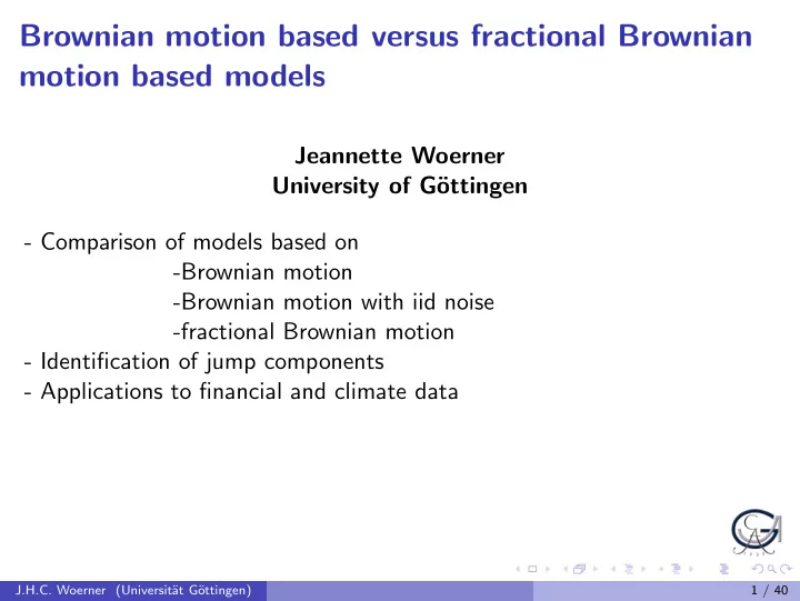
Brownian motion based versus fractional Brownian motion based models Jeannette Woerner University of G ottingen - Comparison of models based on -Brownian motion -Brownian motion with iid noise -fractional Brownian motion - Identification
Brownian motion based versus fractional Brownian motion based models Jeannette Woerner University of G¨ ottingen - Comparison of models based on -Brownian motion -Brownian motion with iid noise -fractional Brownian motion - Identification of jump components - Applications to financial and climate data J.H.C. Woerner (Universit¨ at G¨ ottingen) 1 / 40
Motivation J.H.C. Woerner (Universit¨ at G¨ ottingen) 2 / 40
Motivation discrete data X t n , 0 , · · · , X t n , n t n , n = t =fixed, ∆ n , i → 0 as n → ∞ Assume stochastic volatility model � t X t = Y t + σ s dB s + δ Z t 0 � t X t = Y t + σ s dL s + δ Z t 0 � t σ s dB H X t = Y t + s + δ Z t . 0 Aim: Determine which model is suitable for a specific data set. � t 0 σ 2 Estimate s ds . J.H.C. Woerner (Universit¨ at G¨ ottingen) 3 / 40
� t 0 σ 2 How can we infer s ds First we consider Brownian motion based models . Use the concept of quadratic variation , i.e. realized volatility � t i � t p � σ s dB s | 2 σ 2 | Y t i − Y t i − 1 + → s ds 0 t i − 1 i Advantages: - almost model free, only need some Brownian motion based model - very simple to compute - distributional theory is known and Gaussian J.H.C. Woerner (Universit¨ at G¨ ottingen) 4 / 40
Empirical studies versus theoretical results Statistical principle: Use all available data. Problem: For tick-by-tick data realized volatility increases. Possible Explanation: Market microstructure or market friction i.e. effects due to bid-ask bounces, discreteness of prices, liquidity problems, asymmetric information,... J.H.C. Woerner (Universit¨ at G¨ ottingen) 5 / 40
Model with iid noise (cf. Ait-Sahalia, Mykland and Zhang (2006)) � t X t = σ s dB s + ǫ t , 0 where ǫ denotes iid noise. Then the realized volatility is of the order 2∆ − 1 E ( ǫ 2 ) , hence the noise term leads to a bias with dominates the quadratic variation estimate for small ∆. J.H.C. Woerner (Universit¨ at G¨ ottingen) 6 / 40
J.H.C. Woerner (Universit¨ at G¨ ottingen) 7 / 40
J.H.C. Woerner (Universit¨ at G¨ ottingen) 8 / 40
Non-normed and normed power variation � t V n p ( σ s dB s ) = 0 0 : p > 2 � t i � t p � σ s dB s | p 0 σ 2 | → : p = 2 s ds t i − 1 ∞ : p < 2 i � t � t p ∆ 1 − p / 2 V n σ p p ( σ s dB s ) → µ p s ds , 0 0 as n → ∞ , where µ p = E ( | u | p ) with u ∼ N (0 , 1) and ∆ = t i − t i − 1 . (cf. Barndorff-Nielsen and Shephard (2003)) J.H.C. Woerner (Universit¨ at G¨ ottingen) 9 / 40
Power variation for the model with iid noise Using Minkowski’s inequality with p > 1 we obtain � t i | ǫ t i − ǫ t i − 1 | p ) 1 / p − ( σ s dB s | p ) 1 / p ≤ ( � � � | X t i − X t i − 1 | p ) 1 / p ( | t i − 1 � t i | ǫ t i − ǫ t i − 1 | p ) 1 / p + ( � � σ s dB s | p ) 1 / p ≤ ( | t i − 1 Hence if E | ǫ | p < ∞ for some p > 2, then | X t i − X t i − 1 | p → ∞ , � which does not coincide with empirical findings. J.H.C. Woerner (Universit¨ at G¨ ottingen) 10 / 40
J.H.C. Woerner (Universit¨ at G¨ ottingen) 11 / 40
J.H.C. Woerner (Universit¨ at G¨ ottingen) 12 / 40
Fractional Brownian Motion A fractional Brownian motion (fBm) with Hurst parameter H ∈ (0 , 1), B H = { B H t , t ≥ 0 } is a zero mean Gaussian process with the covariance function s ) = 1 2( t 2 H + s 2 H − | t − s | 2 H ) , E ( B H t B H s , t ≥ 0 . The fBm is a self-similar process, that is, for any constant a > 0, the processes { a − H B H at , t ≥ 0 } and { B H t , t ≥ 0 } have the same distribution. 2 , B H coincides with the classical Brownian motion. For For H = 1 H ∈ ( 1 2 , 1) the process possesses long memory and for H ∈ (0 , 1 2 ) the behaviour is chaotic. J.H.C. Woerner (Universit¨ at G¨ ottingen) 13 / 40
Non-normed Power Variation for fractional Brownian motion 0 : p > 1 / H � t i � t p � 0 σ 1 / H σ s dB H s | p | → , µ 1 / H ds : p = 1 / H s t i − 1 ∞ : p < 1 / H i The integral is a pathwise Riemann-Stieltjes integral and we need that 1 σ is a stochastic process with paths of finite q -variation, q < 1 − H . Idea: Empirical behaviour of tick-by-tick data may also be explained by fBB with H < 0 . 5. J.H.C. Woerner (Universit¨ at G¨ ottingen) 14 / 40
Consistency joint with J.M. Corcuera and D. Nualart (2006) Theorem Suppose that σ t is a stochastic process with finite q-variation, where 1 q < 1 − H . Set � t σ s dB H Z t = s . 0 Then, � T P ∆ 1 − pH V n | σ s | p ds , p ( Z ) − → µ p 0 as n → ∞ . J.H.C. Woerner (Universit¨ at G¨ ottingen) 15 / 40
Estimate for quadratic variation We can explain the empirical findings by considering | X t i − X t i − 1 | 2 = ∆ 2 H − 1 (∆ 1 − 2 H � � | X t i − X t i − 1 | 2 ) , i i where � t p ∆ 1 − 2 H � | X t i − X t i − 1 | 2 σ 2 → s ds 0 i and ∆ 2 H − 1 → ∞ for H < 0 . 5. J.H.C. Woerner (Universit¨ at G¨ ottingen) 16 / 40
More details: We look at the test statistics: � [ nT ] − 1 ( X i +1 n − X i n )( X i n − X i − 1 n ) i =1 S = � [ nT ] n ) 2 i =1 ( X i n − X i − 1 model based on Brownian motion: 0 model based on Brownian motion with iid noise: -1/2 2 (2 2 H − 2) 1 model based on fractional Brownian motion: confidence interval: � � � [ nt ] � [ nt ] n | 4 n | 4 � i =1 | X i n − X i − 1 � i =1 | X i n − X i − 1 � � − c γ � 2 , c γ , � � � 2 � �� [ nt ] � �� [ nt ] n | 2 n | 2 3 i =1 | X i n − X i − 1 3 i =1 | X i n − X i − 1 where c γ denotes the γ -quantile of a N (0 , 1)-distributed random variable. J.H.C. Woerner (Universit¨ at G¨ ottingen) 17 / 40
Daimler Chrysler, January 3rd-31st 2005, 1% level # transactions mean distance S l. bound BM 66140 7s -0.1061 -0.0796 33070 14s -0.1606 -0.1094 22046 21s -0.1574 -0.1244 16535 28s -0.1192 -0.1295 13228 35s -0.1156 -0.1367 # transactions mean distance R l. bound BM 66140 7s -0.424 -0.0357 33070 14s -0.4411 -0.0405 22046 21s -0.3837 -0.0622 16535 28s -0.2744 -0.0467 13228 35s -0.2532 -0.0518 11023 42s -0.2202 -0.0597 9448 49s -0.1749 -0.0601 8267 56s -0.1117 -0.0675 7348 63s -0.1336 -0.0623 6614 70s -0.0972 -0.0702 J.H.C. Woerner (Universit¨ at G¨ ottingen) 18 / 40
Model with market microstructure Daimler Chrysler, January 3rd-31st 2005, 1% level # transactions mean distance S u. bound iid 66140 7s -0.1061 -0.3621 33070 14s -0.1606 -0.3106 22046 21s -0.1574 -0.2845 16535 28s -0.1192 -0.2758 13228 35s -0.1156 -0.2632 11023 42s -0.0994 -0.2413 9448 49s -0.0827 -0.2354 8267 56s -0.0542 -0.2472 7348 63s -0.0608 -0.2134 6614 70s -0.0487 -0.2285 J.H.C. Woerner (Universit¨ at G¨ ottingen) 19 / 40
What are the effects of these results? Risk induced by model misspecification We look at Daimler Chrysler data of 12.1.2005: Assuming a model based on Brownian motion : � T 0 σ 2 s ds = 0 . 000309 Assuming a model based on fractional Brownian motion with H = 0 . 4: � T 0 σ 2 s ds = 0 . 000059 J.H.C. Woerner (Universit¨ at G¨ ottingen) 20 / 40
J.H.C. Woerner (Universit¨ at G¨ ottingen) 21 / 40
What are the effects of these results? Risk induced by model misspecification We look at index data from Singapore: Assuming a model based on Brownian motion : � T 0 σ 2 s ds = 0 . 319 Assuming a model based on fractional Brownian motion with H = 0 . 6: � T 0 σ 2 s ds = 1 . 595 J.H.C. Woerner (Universit¨ at G¨ ottingen) 22 / 40
Do we have an additional jump component? A measure for the activity of the jump component of a L´ evy process is the Blumenthal-Getoor index β , � (1 ∧ | x | δ ) ν ( dx ) < ∞} . β = inf { δ > 0 : This index ensures, that for p > β the sum of the p -th power of jumps will be finite. J.H.C. Woerner (Universit¨ at G¨ ottingen) 23 / 40
Comparison of non-normed power variation 0 : p > 2 � t i � t p � σ s dB s | p 0 σ 2 | → s ds : p = 2 t i − 1 ∞ : p < 2 i and the case for the L´ evy model � t i � σ s dL s | p | t i − 1 i � u u − σ s dL s | p : 0 < u ≤ t ) � � ( | : p > β p → ∞ : p < β under appropriate regularity conditions, where β denotes the Blumenthal-Getoor index of L . J.H.C. Woerner (Universit¨ at G¨ ottingen) 24 / 40
Non-normed Power Variation for fractional Brownian motion 0 : p > 1 / H � t i � t p � σ s dB H s | p 0 σ 1 / H | → , µ 1 / H : p = 1 / H ds s t i − 1 ∞ : p < 1 / H i where H > 1 / 2. The integral is a pathwise Riemann-Stieltjes integral and we need that σ is a stochastic process with paths of finite q -variation, 1 q < 1 − H . Hence one over the Hurst exponent plays a similar role as the Blumenthal-Getoor index . J.H.C. Woerner (Universit¨ at G¨ ottingen) 25 / 40
Recommend
More recommend
Explore More Topics
Stay informed with curated content and fresh updates.
