Variations and Brownian Motion with drift Bo Friis Nielsen 1 1 DTU - PowerPoint PPT Presentation

Variations and Brownian Motion with drift Bo Friis Nielsen 1 1 DTU Informatics 02407 Stochastic Processes 12, November 27 2018 Bo Friis Nielsen Variations and Brownian Motion with drift

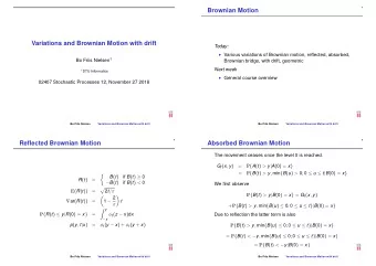
Brownian Motion Today: ◮ Various variations of Brownian motion, reflected, absorbed, Brownian bridge, with drift, geometric Next week ◮ General course overview Bo Friis Nielsen Variations and Brownian Motion with drift

Reflected Brownian Motion � B ( t ) if B ( t ) ≥ 0 R ( t ) = − B ( t ) if B ( t ) < 0 � E ( R ( t )) = 2 t /π � 1 − 2 � V ar ( R ( t )) = t π � y P { R ( t ) ≤ y | R ( 0 ) = x } = φ t ( z − x ) d x − y p ( y , t | x ) = φ t ( y − x ) + φ t ( y + x ) Bo Friis Nielsen Variations and Brownian Motion with drift

Absorbed Brownian Motion The movement ceases once the level 0 is reached. G t ( x , y ) = P { A ( t ) > y | A ( 0 ) = x } = P { B ( t ) > y , min { B ( u ) > 0 ; 0 ≤ u ≤ t | B ( 0 ) = x } We first observe P { B ( t ) > y | B ( 0 ) = x } = G t ( x , y ) + P { B ( t ) > y , min { B ( u ) ≤ 0 ; 0 ≤ u ≤ t }| B ( 0 ) = x } Due to reflection the latter term is also P { B ( t ) > y , min { B ( u ) ≤ 0 ; 0 ≤ u ≤ t }| B ( 0 ) = x } = P { B ( t ) < − y , min { B ( u ) ≤ 0 ; 0 ≤ u ≤ t }| B ( 0 ) = x } = P { B ( t ) < − y | B ( 0 ) = x } Bo Friis Nielsen Variations and Brownian Motion with drift

Absorbed Brownian Motion Summarizing we get P { A ( t ) > y | A ( 0 ) = x } = G t ( x , y ) = 1 − Φ t ( y − x ) − Φ t ( − y − x ) = Φ t ( y + x ) − Φ t ( y − x ) We have already seen that P { A ( t ) = 0 | A ( 0 ) = x } = 2 [ 1 − Φ t ( x )] Bo Friis Nielsen Variations and Brownian Motion with drift

Brownian Bridge Distribution of B ( t ); 0 ≤ t ≤ 1 conditioned on { B ( 0 ) = 0 , B ( 1 ) = 0 } . X = B ( t ) and B ( 1 ) − B ( t ) are indepedent normal variables. Y = B ( 1 ) − B ( t ) + B ( t ) and X are bivariate normal. V ar ( x ) = t √ √ C ov ( X , Y ) = E ( B ( t ) B ( t ) + B ( t )( 1 − B ( t ))) = t = ρ t 1 E ( X ) + ρσ X E ( X | Y = y = 0 ) = · ( y − E ( Y )) = 0 σ Y t ( 1 − ρ 2 ) = t ( 1 − t ) V ar ( X | Y ) = E { B ( t ) | B ( 0 ) = 0 , B ( 1 ) = 0 } = 0 V ar { B ( t ) | B ( 0 ) = 0 , B ( 1 ) = 0 } = t ( 1 − t ) C ov { B ( s ) , B ( t ) | B ( 0 ) = 0 , B ( 1 ) = 0 } = s ( 1 − t ) The process is Gaussian Bo Friis Nielsen Variations and Brownian Motion with drift

Brownian Motion with Drift X ( t ) = µ t + σ B ( t ) ◮ A continuous sample path process with independent increments ◮ X ( t + s ) − X ( s ) ∼ N � µ t , σ 2 t � � y − µ t − x � P { X ( t ) ≤ y | X ( 0 ) = x } = Φ √ σ t Bo Friis Nielsen Variations and Brownian Motion with drift

Absorption Probabilities T ab = min { t ≥ 0 ; X ( t ) = a or X ( t ) = b } u ( x ) = P { X ( T ab ) = b | X ( 0 ) = x } We assume that absorption has not occurred at (∆ t , x + ∆ X ) u ( x ) = E ( u ( x + ∆ X )) Taylor series expansion of right hand side � (∆ X ) 2 �� u ( x ) + u ′ ( x )∆( X ) + 1 2 u ”( x )(∆ X ) 2 + o � u ( x ) = E u ( x ) + u ′ ( x ) E [∆( X )] + 1 � (∆ X ) 2 � � � (∆ X ) 2 �� = 2 u ”( x ) E + E o � (∆ X ) 2 � = σ 2 ∆ t + ( µ ∆ t ) 2 E [∆( X )] = µ ∆ t , E µ u ′ ( x ) + 1 u ( x ) = Ae − 2 µ x 2 σ 2 u ”( x ) = 0 , σ 2 + B Bo Friis Nielsen Variations and Brownian Motion with drift

Absorption probabilities Theorem 8.1 µ u ′ ( x ) + 1 u ( x ) = Ae − 2 µ x σ 2 + B 2 σ 2 u ”( x ) = 0 , u ( x ) = Ae − 2 µ x σ 2 + B , u ( a ) = 0 , u ( b ) = 1 u ( x ) = e − 2 µ x σ 2 − e − 2 µ a σ 2 e − 2 µ b σ 2 − e − 2 µ a σ 2 Bo Friis Nielsen Variations and Brownian Motion with drift

Mean Time to Absorption T ab = min { t ≥ 0 ; X ( t ) = a or X ( t ) = b } v ( x ) = E { T ab | X ( 0 ) = x } v ( x ) = ∆ t + E ( v ( x + ∆ X )) 1 + µ v ′ ( x ) + 1 2 σ 2 v ”( x ) = 0 v ( a ) = v ( b ) = 0 v ( x ) = 1 µ [ u ( x )( b − a ) − ( x − a )] Bo Friis Nielsen Variations and Brownian Motion with drift

Maximum of Brownian Motion with Negative Drift We assume µ < 0, using Theorem 8.2.1 u ( x ) = e − 2 µ x σ 2 − e − 2 µ a σ 2 e − 2 µ b σ 2 − e − 2 µ a σ 2 we get e − 2 µ · 0 σ 2 − e − 2 µ a σ 2 = e − 2 | µ | σ 2 y P { max 0 ≤ t X ( t ) > y } = lim e − 2 µ y σ 2 − e − 2 µ a a →−∞ σ 2 Bo Friis Nielsen Variations and Brownian Motion with drift

Geometric Brownian Motion Z ( t ) = ze ( α − 1 2 σ 2 ) t + σ B ( t ) ( Z ( 0 ) = z ) � α − 1 � 2 σ 2 , σ 2 X ( t ) = log ( z ) + log ( Z ( t ) , X ( t ) ∼ N 2 σ 2 ) t = ze α t E ( Z ( t )) = ze ( α − 1 2 σ 2 ) t E � e σ B ( t ) � = ze ( α − 1 2 σ 2 ) t e ( 1 2 σ 2 we have that Z ( t ) → 0 with probability 1 For α < 1 e σ 2 t − 1 V ar ( Z ( t )) = z 2 e 2 α t � � Bo Friis Nielsen Variations and Brownian Motion with drift