Lecture 5: Convolution Princeton University COS 495 Instructor: - PowerPoint PPT Presentation

Deep Learning Basics Lecture 5: Convolution Princeton University COS 495 Instructor: Yingyu Liang

Convolutional neural networks • Strong empirical application performance • Convolutional networks: neural networks that use convolution in place of general matrix multiplication in at least one of their layers ℎ = 𝜏(𝑋 𝑈 𝑦 + 𝑐) for a specific kind of weight matrix 𝑋

Convolution

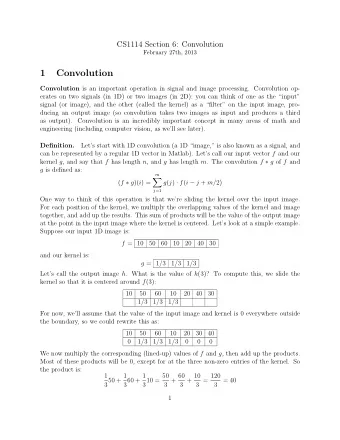
Convolution: math formula • Given functions 𝑣(𝑢) and 𝑥(𝑢) , their convolution is a function 𝑡 𝑢 𝑡 𝑢 = ∫ 𝑣 𝑏 𝑥 𝑢 − 𝑏 𝑒𝑏 • Written as 𝑡 = 𝑣 ∗ 𝑥 or 𝑡 𝑢 = (𝑣 ∗ 𝑥)(𝑢)

Convolution: discrete version • Given array 𝑣 𝑢 and 𝑥 𝑢 , their convolution is a function 𝑡 𝑢 +∞ 𝑡 𝑢 = ෍ 𝑣 𝑏 𝑥 𝑢−𝑏 𝑏=−∞ • Written as 𝑡 = 𝑣 ∗ 𝑥 or 𝑡 𝑢 = 𝑣 ∗ 𝑥 𝑢 • When 𝑣 𝑢 or 𝑥 𝑢 is not defined, assumed to be 0

Illustration 1 𝑥 = [z, y, x] 𝑣 = [a, b, c, d, e, f] xb+yc+zd x y z a b c d e f

Illustration 1 xc+yd+ze x y z a b c d e f

Illustration 1 xd+ye+zf x y z a b c d e f

Illustration 1: boundary case xe+yf x y a b c d e f

Illustration 1 as matrix multiplication y z a x y z b x y z c x y z d x y z e x y f

Illustration 2: two dimensional case a b c d w x e f g h y z i j k l wa + bx + ey + fz

Illustration 2 a b c d w x e f g h y z i j k l wa + bx + bw + cx + ey + fz fy + gz

Illustration 2 Input Kernel (or filter) a b c d w x e f g h y z i j k l wa + bx + bw + cx + ey + fz fy + gz Feature map

Advantage: sparse interaction Fully connected layer, 𝑛 × 𝑜 edges 𝑛 output nodes 𝑜 input nodes Figure from Deep Learning, by Goodfellow, Bengio, and Courville

Advantage: sparse interaction Convolutional layer, ≤ 𝑛 × 𝑙 edges 𝑛 output nodes 𝑙 kernel size 𝑜 input nodes Figure from Deep Learning, by Goodfellow, Bengio, and Courville

Advantage: sparse interaction Multiple convolutional layers: larger receptive field Figure from Deep Learning, by Goodfellow, Bengio, and Courville

Advantage: parameter sharing The same kernel are used repeatedly. E.g., the black edge is the same weight in the kernel. Figure from Deep Learning, by Goodfellow, Bengio, and Courville

Advantage: equivariant representations • Equivariant: transforming the input = transforming the output • Example: input is an image, transformation is shifting • Convolution(shift(input)) = shift(Convolution(input)) • Useful when care only about the existence of a pattern, rather than the location

Pooling

Terminology Figure from Deep Learning, by Goodfellow, Bengio, and Courville

Pooling • Summarizing the input (i.e., output the max of the input) Figure from Deep Learning, by Goodfellow, Bengio, and Courville

Advantage Induce invariance Figure from Deep Learning, by Goodfellow, Bengio, and Courville

Motivation from neuroscience • David Hubel and Torsten Wiesel studied early visual system in human brain (V1 or primary visual cortex), and won Nobel prize for this • V1 properties • 2D spatial arrangement • Simple cells: inspire convolution layers • Complex cells: inspire pooling layers

Variants of convolution and pooling

Variants of convolutional layers • Multiple dimensional convolution • Input and kernel can be 3D • E.g., images have (width, height, RBG channels) • Multiple kernels lead to multiple feature maps (also called channels) • Mini-batch of images have 4D: (image_id, width, height, RBG channels)

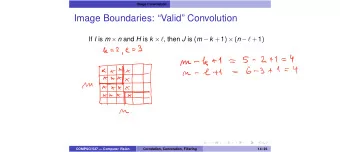
Variants of convolutional layers • Padding: valid xd+ye+zf x y z a b c d e f

Variants of convolutional layers • Padding: same xe+yf x y a b c d e f

Variants of convolutional layers • Stride Figure from Deep Learning, by Goodfellow, Bengio, and Courville

Variants of convolutional layers • Others: • Tiled convolution • Channel specific convolution • ……

Variants of pooling • Stride and padding Figure from Deep Learning, by Goodfellow, Bengio, and Courville

Variants of pooling • Max pooling 𝑧 = max{𝑦 1 , 𝑦 2 , … , 𝑦 𝑙 } • Average pooling 𝑧 = mean{𝑦 1 , 𝑦 2 , … , 𝑦 𝑙 } • Others like max-out