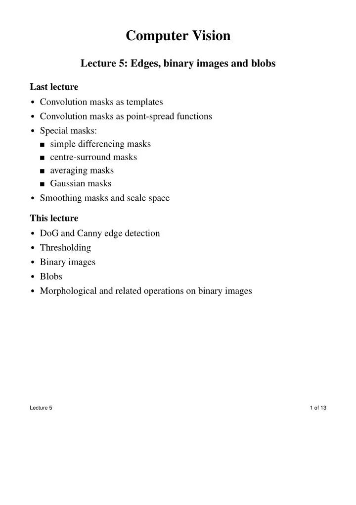
Computer Vision Lecture 5: Edges, binary images and blobs Last - PDF document

Computer Vision Lecture 5: Edges, binary images and blobs Last lecture • Convolution masks as templates • Convolution masks as point-spread functions • Special masks: ■ simple differencing masks ■ centre-surround masks ■ averaging masks ■ Gaussian masks • Smoothing masks and scale space This lecture • DoG and Canny edge detection • Thresholding • Binary images • Blobs • Morphological and related operations on binary images Lecture 5 1 of 13

Edge detection Edge detection requires • a spatial scale, established using a smoothing operator • a differencing operator to find significant grey-level changes The Difference of Gaussians mask A classical, biologically-inspired approach is to combine Gaussian smoothing with a centre-surround operator. The two masks can be combined by convolution into a single one. Mathematically this leads to a mask called the Laplacian of the Gaussian mask. In practice, it is almost always approximated using the Difference of Gaussians or DoG mask. -1/8 -1/8 -1/8 * -1/8 +1 -1/8 -1/8 -1/8 -1/8 convolve - (approximately) Note that larger Gaussian masks have smaller values at the centre. Lecture 5 2 of 13

The DoG mask is circularly symmetrical. A profile through the middle looks like this, and it is sometimes called the Mexican hat operator: The DoG picks out structure at a particular scale. Here σ is 1 and 2. Lecture 5 3 of 13

The edge detector closely associated with David Marr then detects the zero- crossings of the convolved images. Zero-crossings are the points where negative and positive pixels are adjacent. In the images below, the zero-crossings are at the boundaries of the black (or white) areas. Marr went on to propose that meaningful image boundaries occurred when the zero-crossings at different scales coincide. Marr’s book Vision is a key reference in this area. Lecture 5 4 of 13

Gaussian derivative masks In fact, the most popular masks used for Computer Vision are those that combine the simple directional operators with Gaussian smoothing. These tend to produce more robust results than the DoG. * = -1 +1 -1 * = +1 Such masks emphasise vertical and horizontal structure at the scale set by the σ parameter of the Gaussian component. The upper mask is the horizontal or x derivative, the lower one the vertical or y derivative. These outputs are also called the gradients in the x and y directions, estimated at the scale σ . Convolutions with both DoG and Gaussian derivative masks can be computed efficiently by separating them out into pairs of 1-dimensional masks. This property — separability — is specific to certain masks only. Lecture 5 5 of 13

The Canny edge detector One of the most popular edge detectors of recent years, developed by Canny, uses the outputs of two Gaussian derivative masks. The two outputs are combined by squaring and adding. The peaks of ridges are then found. Ridges that contain a peak over a given threshold are retained as long as they stay above another, lower threshold. x gradient square and add threshold y gradient Lecture 5 6 of 13

Canny’s merits are more obvious when applied to an image of a less natural object. The brighter the line in the image, the stronger the edge strength. The scale parameter and thresholds chosen affect the density and accuracy of the edges found by this edge detector. Lecture 5 7 of 13

Review of thresholding Setting each pixel greater than a certain threshold to one value, and all the other pixels to the other value, is the simplest way to produce a binary image Applied to ordinary grey-level images, this is not very useful because of variations in lighting and intrinsic surface brightness. Automatic setting of the threshold can help. It can be useful applied to raw images in certain industrial settings — e.g. printed circuit board inspection. It is often useful when applied to the outputs of convolutions, since differencing operators take away the overall brightness variations, leaving contrasts. Multi-level thresholding can also be useful. This is closely related to image quantisation as used for some graphics effects. Lecture 5 8 of 13

Binary images DoG and Canny edge detection conform to the structure of most “early” or “low-level” visual processing: • one or more convolutions (linear operations), followed by • some non-linear operations, such as squaring and thresholding. If the final operation is thresholding, this leads to a binary image in which features such as edges are marked. Binary images contain only 2 values, often 0 and 1. (When they are displayed, the non-zero parts may be black or white.) Here the black lines are the non-zero pixels in the Canny edge-detected image. Lecture 5 9 of 13

Connected regions in binary images A connected region is a collected of non-zero pixels which join onto one another. I often call such a region a blob . Two non-zero pixels are in the same region if you can get from one to the other by making jumps to neighbouring pixels without going onto a zero pixel. 0 0 0 0 0 0 0 0 0 0 0 0 1 1 1 0 0 1 0 0 0 0 0 0 1 1 1 1 0 0 1 1 0 0 0 1 1 0 1 1 0 1 1 0 0 0 0 0 0 0 0 0 0 0 0 0 1 0 1 0 0 0 0 0 0 0 0 1 1 1 0 0 0 1 0 1 0 0 0 0 0 0 0 0 0 1 0 0 0 0 0 0 0 0 0 0 0 0 0 This binary image has 4 blobs under 8-connectivity but 7 blobs under 4- connectivity. Blob finding algorithms come in two kinds: • Recursive. Starting from a non-zero pixel: ■ 1. find all the unmarked non-zero neighbours and mark them as visited; ■ 2. for each of these neighbours, go to step 1. • Iterative. Scan the array in raster-scan order; when a non-zero pixel is reached, look above and to the left for other non-zero pixels, and if one is found, join the current pixel to this blob. Join blobs at the bottom of “U”s. Lecture 5 10 of 13

Blob measurements Blobs can be characterised using a variety of measurements major axis orientation area minor axis perimeter • aspect ratio is ratio of major to minor axis • compactness can be measured by ratio of area to (perimeter squared) and for simple segmentations it is very easy to get the bounding box See the imfeature function in Matlab. Details are in the Image Processing User’s Guide. Lecture 5 11 of 13

Morphological operations It may be useful to operate on the shape of a blob (as opposed to the grey levels of the image). Dilation grows a blob by adding adjoining pixels to it. This smooths the shape and can merge nearby blobs. (The example uses 8-connectivity.) Erosion shrinks a blob by removing pixels that are adjacent to non-zero pixels. This removes small blobs entirely. Sequences of dilation and erosion operations can provide powerful tools. Lecture 5 12 of 13

Dilation and erosion can be defined more generally using a structuring element . This is a binary mask which is slide over the image, convolution- fashion. Whenever it overlaps a “1” pixel in the input, a 1 is written to the relevant output pixel. Thinning Thinning and skeletonisation are similar to erosion but preserve connectivity — one application is in handwriting analysis. Various algorithms exist — consult e.g. Ballard & Brown or Gonzalez & Wintz (see bibliography), or the Matlab Image Processing Toolbox User’s Guide (under binary image operations). (It is not trivial to do skeletonisation efficiently and correctly.) Lecture 5 13 of 13