CS 4495 Computer Vision 3D Perception Kelsey Hawkins Robotics 3D - PowerPoint PPT Presentation
3D Perception CS 4495 Computer Vision K. Hawkins CS 4495 Computer Vision 3D Perception Kelsey Hawkins Robotics 3D Perception CS 4495 Computer Vision K. Hawkins Motivation What do animals, people, and robots want to do with vision?
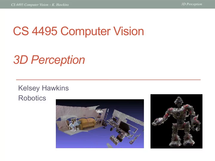
3D Perception CS 4495 Computer Vision – K. Hawkins CS 4495 Computer Vision 3D Perception Kelsey Hawkins Robotics
3D Perception CS 4495 Computer Vision – K. Hawkins Motivation What do animals, people, and robots want to do with vision? ● Detect and recognize objects/landmarks ● Is that a banana or a snake? A cup or a plate? – Find location of objects with respect to themselves ● Want to grasp fruit/tool, where should I put my body/arm? – Changes in elevation: steps, rocks, inclined planes – Determine shape ● What is the physical 3D structure of this object? – Where does an object begin and the background begin? – Find obstacles and map the environment ● – How do I get my body/arm from A to B without hitting things? Others – tracking, dynamics, etc. ●
3D Perception CS 4495 Computer Vision – K. Hawkins Weaknesses of Images Surface Geometry Color Inconsistency
3D Perception CS 4495 Computer Vision – K. Hawkins Weaknesses of Monocular Vision Scale Lack of texture Background-foreground similarity
3D Perception CS 4495 Computer Vision – K. Hawkins Potential solution: 3D Sensing pointclouds.org
3D Perception CS 4495 Computer Vision – K. Hawkins Types of 3D Sensing ● Passive 3D sensing – Work with naturally occurring light – Exploit geometry or known properties of scenes ● Active 3D sensing – Project light or sound out into the environment and see how it reacts – Encode some pattern which can be found in the sensor
3D Perception CS 4495 Computer Vision – K. Hawkins Passive – 3D Sensors Stereo Rigs Shape from focus Nayar, Watanabe, and Noguchi 1996
3D Perception CS 4495 Computer Vision – K. Hawkins Active – Photometric Stereo
3D Perception CS 4495 Computer Vision – K. Hawkins Active – Time of Flight ● Bounce signal off of a surface, record time to come back, X=V*t/2 LIDAR / Laser / SONAR / Sound / Range finder Transceiver
3D Perception CS 4495 Computer Vision – K. Hawkins Active - Structured Light ● Remember stereo? ● Let's replace the camera with a projector ● Instead of looking for the same features in both image, we look for a known feature we've projected on the scene
3D Perception CS 4495 Computer Vision – K. Hawkins Active – Structured Light Zhang, Li et. al. "Rapid shape acquisition..."
3D Perception CS 4495 Computer Vision – K. Hawkins Active – Infrared Structured Light
3D Perception CS 4495 Computer Vision – K. Hawkins How the Kinect works ● Cylindrical lens – Only focuses light in one direction PrimeSense patent 2010/0290698
3D Perception CS 4495 Computer Vision – K. Hawkins How the Kinect works PrimeSense patent No. 20100290698
3D Perception CS 4495 Computer Vision – K. Hawkins How the Kinect works PrimeSense patent No. 20100290698
3D Perception CS 4495 Computer Vision – K. Hawkins How the Kinect works PrimeSense patent 2010/0290698
3D Perception CS 4495 Computer Vision – K. Hawkins How the Kinect works Psuedo-random speckle pattern PrimeSense patent 2010/0290698
3D Perception CS 4495 Computer Vision – K. Hawkins 2D vs. 3D Perception 2D 3D Analysis Tools ● Depth image (u,v,d) Representation Image (u,v) ● Point cloud (x,y,z) 1st order differential Image gradients Surface normals geometry 2nd order differential Second moment matrix Principle curvature geometry Corner detection Harris image Surface variation ● Point Feature Feature extraction HOG Histograms ● Spin Images Geometric model Hough transform Clustering + RANSAC fitting Iterative Closest Point Alignment SSD window filter (ICP)
3D Perception CS 4495 Computer Vision – K. Hawkins Depth Images ● Advantages – Dense representation – Gives intuition about occlusion and free space – Depth discontinuities are just edges on the image ● Disadvantages – Viewpoint dependent, can't merge – Doesn't capture physical geometry – Need actual 3D locations
3D Perception CS 4495 Computer Vision – K. Hawkins Point Clouds ● Take every depth pixel and put it out in the world ● What can this representation tell us? ● What information do we lose? R. Rusu's PCL Presentation
3D Perception CS 4495 Computer Vision – K. Hawkins Point Clouds ● Advantages – Viewpoint independent – Captures surface geometry – Points represent physical locations ● Disadvantages – Sparse representation – Lost information about free space and unknown space – Variable density based on distance from sensor R. Rusu's PCL Presentation
3D Perception CS 4495 Computer Vision – K. Hawkins Point Clouds and Surfaces ● Point clouds are sampled from the surfaces of the objects perceived ● The concept of volume is inferred, not perceived
3D Perception CS 4495 Computer Vision – K. Hawkins Surfaces ● Let's say we'd like to learn the “geometry” around a point in our cloud ● What is the simplest surface representation we could use to approximate the surface about a point? ● Tangent plane – Defined by normal ● First-order approximation
3D Perception CS 4495 Computer Vision – K. Hawkins Surfaces ● To understand how we can characterise surfaces, we can look to differential geometry ● A surface is 2D manifold in 3D space f : ℝ 2 →ℝ 3 f ( u,v )=( x , y ,z ) ● Parametric representation ● How u and v are “oriented” with respect to the surface is irrelevant
3D Perception CS 4495 Computer Vision – K. Hawkins Surfaces v u
3D Perception CS 4495 Computer Vision – K. Hawkins Surfaces v u
3D Perception CS 4495 Computer Vision – K. Hawkins Surfaces v u
3D Perception CS 4495 Computer Vision – K. Hawkins Surface Normals ● Want to estimate this function f ( u,v ) ● What can we do to estimate this function? Taylor Series 1st order approximation at ( u 0, v 0 ) f ( u,v )≈ f ( u 0, v 0 )+[ u − u 0, v − v 0 ] [ ∂ v ( u 0, v 0 ) ] ∂ f ∂ u ( u 0, v 0 ) ∂ f
3D Perception CS 4495 Computer Vision – K. Hawkins Surface Normals ● We have a problem though... ( u, v ) ● Don't have basis, infinite exist! ● Take a sample of 3D points we believe f ( u,v ) ( u 0, v 0 ) lie on around u n − u 0 v n − v 0 ] [ T ] ∂ f A = [ f ( u n ,v n ) ] = [ x n y n z n ] = [ T ∂ u ( u 0, v 0 ) f ( u 1, v 1 ) x 1 y 1 z 1 u 1 − u 0 v 1 − v 0 ⋮ ⋮ ⋮ ∂ f ∂ v ( u 0, v 0 ) ● Find n such that An = 0 ● We've done this before (last eigenvector)
3D Perception CS 4495 Computer Vision – K. Hawkins Surface Normals u n − u 0 v n − v 0 ] [ T ] n = 0 ⇔ [ T ] T T ∂ f ∂ f An = [ u 1 − u 0 v 1 − v 0 n = 0 ⇔ ∂ f ∂ u ⋅ n = 0 , ∂ f ∂ u ∂ u ∂ v ⋅ n = 0 ⋮ ∂ f ∂ f ∂ v ∂ v ∂ u ⊥ n, ∂ f ∂ f ● This n (the normal) is perpendicular to ∂ v ⊥ n both partials, regardless of basis choice ● Surface normal is a first order approximation of the surface at the point invariant to basis choice
3D Perception CS 4495 Computer Vision – K. Hawkins Surface Normals ● Size of patch is like width of Gaussian in image gradient calculation ● We can use them to find planes
3D Perception CS 4495 Computer Vision – K. Hawkins Principal Curvature ● Second order approximation
3D Perception CS 4495 Computer Vision – K. Hawkins Surface Variation A = [ f ( u n ,v n ) ] = [ x n y n z n ] f ( u 1, v 1 ) x 1 y 1 z 1 ⋮ ⋮ Normal T = U [ s 0 ] s 2 0 0 T [ v 2 v 1 v 0 ] A = U S V s 1 0 0 0 0 2 s 0 Principal surface variation = 2 + s 1 2 + s 2 2 s 0 Curvatures ● This is equivalent to finding the eigenvalues/vectors T A of the covariance matrix A
3D Perception CS 4495 Computer Vision – K. Hawkins Normals / Surface Variation Demo
3D Perception CS 4495 Computer Vision – K. Hawkins Feature Extraction ● Suppose we want a denser description of the local surface function ● Want to find unique patches of surface geometry ● What type of invariance do we need? ● Need viewpoint invariance – Translation + orientation – Color and texture come automatically!
3D Perception CS 4495 Computer Vision – K. Hawkins Point Feature Histograms ● Remember SIFT? ● We're going to use roughly the same idea – Use the normal at the point to establish a dominant orientation – Build a histogram of the orientations of normals in the general region with respect to the original
3D Perception CS 4495 Computer Vision – K. Hawkins Point Feature Histograms ● At a point, take a ball of points around it ● For every pair of points, find the relationship between the two points and their normals ● Must be frame independent R. Rusu's Thesis
3D Perception CS 4495 Computer Vision – K. Hawkins Point Feature Histograms ( x 1, y 1, z 1, n x1 ,n y1 ,n z1 ) ● Reduce to 4 variables ( x 2, y 2, z 2, n x2 ,n y2 ,n z2 ) R. Rusu's Thesis
3D Perception CS 4495 Computer Vision – K. Hawkins Point Feature Histograms ● Find these for variables for every pair in the ball ● Build a 5x5x5x5 histogram of the variables Often the distance variable is excluded – In this case, we have a 125-long feature vector – ● Use this just like a SIFT feature descriptor ● Usually, a sped-up version called Fast Point Feature Histograms is used for real-time applications
Recommend


More recommend
Explore More Topics
Stay informed with curated content and fresh updates.