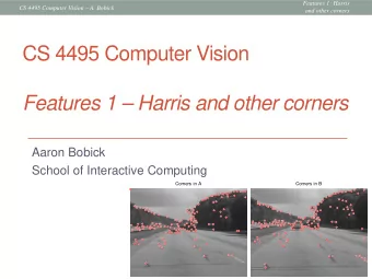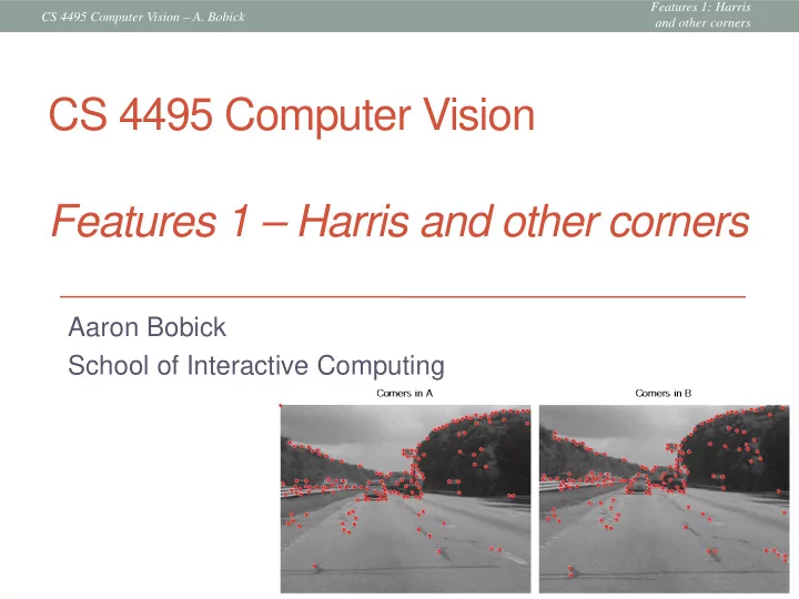
CS 4495 Computer Vision Features 1 Harris and other corners Aaron - PowerPoint PPT Presentation

Features 1: Harris CS 4495 Computer Vision – A. Bobick and other corners CS 4495 Computer Vision Features 1 – Harris and other corners Aaron Bobick School of Interactive Computing

Features 1: Harris CS 4495 Computer Vision – A. Bobick and other corners Administrivia • PS 4: Out and not changed. Due Sunday Oct 12 th , 11:55pm • It is application of the last few lectures. Mostly straight forward Matlab but if you’re linear algebra is rusty it can take a while to figure out. Question 2 takes some doing to understand. • You have been warned… • It is cool • You have been warned… • Today: Start on features. • Forsyth and Ponce: 5.3-5.4 • Szeliski also covers this well – Section 4 – 4.1.1 • These next 3 lectures will provide detail for Project 4.

Features 1: Harris CS 4495 Computer Vision – A. Bobick and other corners The basic image point matching problem • Suppose I have two images related by some transformation. Or have two images of the same object in different positions. • How to find the transformation of image 1 that would align it with image 2?

Features 1: Harris CS 4495 Computer Vision – A. Bobick and other corners We want Local (1) Features (2) • Goal: Find points in an image that can be: • Found in other images • Found precisely – well localized • Found reliably – well matched • Why? • Want to compute a fundamental matrix to recover geometry • Robotics/Vision: See how a bunch of points move from one frame to another. Allows computation of how camera moved -> depth -> moving objects • Build a panorama…

Features 1: Harris CS 4495 Computer Vision – A. Bobick and other corners Suppose you want to build a panorama M. Brown and D. G. Lowe. Recognising Panoramas. ICCV 2003

Features 1: Harris CS 4495 Computer Vision – A. Bobick and other corners How do we build panorama? • We need to match (align) images

Features 1: Harris CS 4495 Computer Vision – A. Bobick and other corners Matching with Features • Detect features (feature points) in both images

Features 1: Harris CS 4495 Computer Vision – A. Bobick and other corners Matching with Features • Detect features (feature points) in both images • Match features - find corresponding pairs

Features 1: Harris CS 4495 Computer Vision – A. Bobick and other corners Matching with Features • Detect features (feature points) in both images • Match features - find corresponding pairs • Use these pairs to align images

Features 1: Harris CS 4495 Computer Vision – A. Bobick and other corners Matching with Features • Problem 1: • Detect the same point independently in both images no chance to match! We need a repeatable detector

Features 1: Harris CS 4495 Computer Vision – A. Bobick and other corners Matching with Features • Problem 2: • For each point correctly recognize the corresponding one ? We need a reliable and distinctive descriptor

Features 1: Harris CS 4495 Computer Vision – A. Bobick and other corners More motivation… • Feature points are used also for: • Image alignment (e.g. homography or fundamental matrix) • 3D reconstruction • Motion tracking • Object recognition • Indexing and database retrieval • Robot navigation • … other

Features 1: Harris CS 4495 Computer Vision – A. Bobick and other corners Characteristics of good features • Repeatability/Precision • The same feature can be found in several images despite geometric and photometric transformations • Saliency/Matchability • Each feature has a distinctive description • Compactness and efficiency • Many fewer features than image pixels • Locality • A feature occupies a relatively small area of the image; robust to clutter and occlusion

Features 1: Harris CS 4495 Computer Vision – A. Bobick and other corners Corner Detection: Basic Idea • We should easily recognize the point by looking through a small window • Shifting a window in any direction should give a large change in intensity “flat” region: “edge”: “corner”: no change in no change significant change all directions along the edge in all directions with direction small shift Source: A. Efros

Features 1: Harris CS 4495 Computer Vision – A. Bobick and other corners Finding Corners • Key property: in the region around a corner, image gradient has two or more dominant directions • Corners are repeatable and distinctive C.Harris and M.Stephens. "A Combined Corner and Edge Detector.“ Proceedings of the 4th Alvey Vision Conference : pages 147—151, 1988

Features 1: Harris CS 4495 Computer Vision – A. Bobick and other corners Finding Harris Corners • Key property: in the region around a corner, image gradient has two or more dominant directions • Corners are repeatable and distinctive C. Harris and M.Stephens. "A Combined Corner and Edge Detector.“ Proceedings of the 4th Alvey Vision Conference : pages 147—151, 1988

Features 1: Harris CS 4495 Computer Vision – A. Bobick and other corners Corner Detection: Mathematics Change in appearance for the shift [ u,v ]: [ ] ∑ 2 = + + − E u v ( , ) w x y ( , ) I x ( u y , v ) I x y ( , ) x y , Window Shifted Intensity function intensity Window function w(x,y) = or 1 in window, 0 outside Gaussian Source: R. Szeliski

Features 1: Harris CS 4495 Computer Vision – A. Bobick and other corners Corner Detection: Mathematics Change in appearance for the shift [ u,v ]: [ ] ∑ 2 = + + − E u v ( , ) w x y ( , ) I x ( u y , v ) I x y ( , ) x y , I ( x , y ) E ( u , v ) E (3,2) E (0,0)

Features 1: Harris CS 4495 Computer Vision – A. Bobick and other corners Corner Detection: Mathematics Change in appearance for the shift [ u,v ]: [ ] ∑ 2 = + + − E u v ( , ) w x y ( , ) I x ( u y , v ) I x y ( , ) x y , We want to find out how this function behaves for small shifts (u,v near 0,0)

Features 1: Harris CS 4495 Computer Vision – A. Bobick and other corners Corner Detection: Mathematics Change in appearance for the shift [ u,v ]: [ ] ∑ 2 = + + − E u v ( , ) w x y ( , ) I x ( u y , v ) I x y ( , ) x y , Second-order Taylor expansion of E ( u , v ) about (0,0) (local quadratic approximation for small u,v ): 2 dF (0) 1 d F (0) δ ≈ + δ + δ 2 (1D ): F ( x ) F ( 0 ) x · x · 2 d x 2 dx       E (0,0) E (0,0) E (0,0) u 1 ≈ + + u uu uv E u v ( , ) E (0,0) [ u v ]   [ u v ]      E (0,0)   E (0,0) E (0,0)    v 2 v uv vv

Features 1: Harris CS 4495 Computer Vision – A. Bobick and other corners Corner Detection: Mathematics [ ] ∑ 2 = + + − E u v ( , ) w x y ( , ) I x ( u y , v ) I x y ( , ) x y , Second-order Taylor expansion of E ( u , v ) about (0,0):       E ( 0 , 0 ) E ( 0 , 0 ) E ( 0 , 0 ) u 1 ≈ + + u uu uv E ( u , v ) E ( 0 , 0 ) [ u v ]   [ u v ]      E ( 0 , 0 )   E ( 0 , 0 ) E ( 0 , 0 )   v  2 v uv vv [ ] ∑ = + + − + + E ( u , v ) 2 w ( x , y ) I ( x u , y v ) I ( x , y ) I ( x u , y v ) u x x , y ∑ = + + + + E ( u , v ) 2 w ( x , y ) I ( x u , y v ) I ( x u , y v ) uu x x x , y [ ] ∑ + + + − + + 2 w ( x , y ) I ( x u , y v ) I ( x , y ) I ( x u , y v ) xx x , y ∑ = + + + + E ( u , v ) 2 w ( x , y ) I ( x u , y v ) I ( x u , y v ) uv y x x , y [ ] ∑ + + + − + + 2 w ( x , y ) I ( x u , y v ) I ( x , y ) I ( x u , y v ) xy x , y

Features 1: Harris CS 4495 Computer Vision – A. Bobick and other corners Corner Detection: Mathematics [ ] ∑ 2 = + + − E u v ( , ) w x y ( , ) I x ( u y , v ) I x y ( , ) x y , Second-order Taylor expansion of E ( u , v ) about (0,0):       E ( 0 , 0 ) E ( 0 , 0 ) E ( 0 , 0 ) u 1 ≈ + + u uu uv E ( u , v ) E ( 0 , 0 ) [ u v ]   [ u v ]      E ( 0 , 0 )   E ( 0 , 0 ) E ( 0 , 0 )   v  2 v uv vv [ ] ∑ = + + − + + E ( u , v ) 2 w ( x , y ) I ( x u , y v ) I ( x , y ) I ( x u , y v ) u x x , y ∑ = + + + + E ( u , v ) 2 w ( x , y ) I ( x u , y v ) I ( x u , y v ) uu x x x , y [ ] ∑ + + + − + + 2 w ( x , y ) I ( x u , y v ) I ( x , y ) I ( x u , y v ) xx x , y ∑ = + + + + E ( u , v ) 2 w ( x , y ) I ( x u , y v ) I ( x u , y v ) uv y x x , y [ ] ∑ + + + − + + 2 w ( x , y ) I ( x u , y v ) I ( x , y ) I ( x u , y v ) xy x , y