CS 4495 Computer Vision Classification 2 Aaron Bobick School of - PowerPoint PPT Presentation

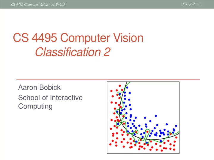
Classifcation2 CS 4495 Computer Vision – A. Bobick K-Nearest Neighbors classification • For a new point, find the k closest points from training data • Labels of the k points “vote” to classify k = 5 Black = negative If query lands here, the 5 Red = positive NN consist of 3 negatives and 2 positives, so we classify it as negative. Source: D. Lowe

Classifcation2 CS 4495 Computer Vision – A. Bobick Discriminative classification methods Discriminative classifiers – find a division (surface) in feature space that separates the classes Several methods • Nearest neighbors • Boosting • Support Vector Machines

Classifcation2 CS 4495 Computer Vision – A. Bobick Discriminative classification methods Discriminative classifiers – find a division (surface) in feature space that separates the classes Several methods • Nearest neighbors • Boosting • Support Vector Machines

Classifcation2 CS 4495 Computer Vision – A. Bobick Boosting: Training method • Initially, weight each training example equally • In each boosting round: • Find the weak learner that achieves the lowest weighted training error • Raise weights of training examples misclassified by current weak learner • Compute final classifier as linear combination of all weak learners (weight of each learner is directly proportional to its accuracy) Slide credit: Lana Lazebnik

Classifcation2 CS 4495 Computer Vision – A. Bobick Boosting intuition Weak Classifier 1 Slide credit: Paul Viola

Classifcation2 CS 4495 Computer Vision – A. Bobick Boosting: Training method • In each boosting round: • Find the weak learner that achieves the lowest weighted training error • Raise weights of training examples misclassified by current weak learner Slide credit: Lana Lazebnik

Classifcation2 CS 4495 Computer Vision – A. Bobick Boosting: Training method • In each boosting round: • Find the weak learner that achieves the lowest weighted training error • Raise weights of training examples misclassified by current weak learner Slide credit: Lana Lazebnik

Classifcation2 CS 4495 Computer Vision – A. Bobick Boosting intuition Weak Classifier 1 Slide credit: Paul Viola

Classifcation2 CS 4495 Computer Vision – A. Bobick Boosting illustration Weights Increased

Classifcation2 CS 4495 Computer Vision – A. Bobick Boosting illustration Weak Classifier 2

Classifcation2 CS 4495 Computer Vision – A. Bobick Boosting illustration Weights Increased

Classifcation2 CS 4495 Computer Vision – A. Bobick Boosting illustration Weak Classifier 3

Classifcation2 CS 4495 Computer Vision – A. Bobick Boosting illustration Final classifier is a combination of weak classifiers

Classifcation2 CS 4495 Computer Vision – A. Bobick Boosting: Training method • Initially, weight each training example equally • In each boosting round: • Find the weak learner that achieves the lowest weighted training error • Raise weights of training examples misclassified by current weak learner • Compute final classifier as linear combination of all weak learners (weight of each learner is directly proportional to its accuracy) • Exact formulas for re-weighting and combining weak learners depend on the particular boosting scheme (e.g., AdaBoost) Slide credit: Lana Lazebnik

Classifcation2 CS 4495 Computer Vision – A. Bobick Viola-Jones face detector

Classifcation2 CS 4495 Computer Vision – A. Bobick Viola-Jones face detector Main ideas: • Represent local texture with efficiently computable “rectangular” features within window of interest • Select discriminative features to be weak classifiers • Use boosted combination of them as final classifier • Form a cascade of such classifiers, rejecting clear negatives quickly Kristen Grauman

Classifcation2 CS 4495 Computer Vision – A. Bobick Viola-Jones detector: features “ Rectangular” filters Feature output is difference between adjacent regions Value at (x,y) is Efficiently computable sum of pixels above and to the with integral image: any left of (x,y) sum can be computed in constant time. Integral image Kristen Grauman

Classifcation2 CS 4495 Computer Vision – A. Bobick Computing sum within a rectangle • Let A,B,C,D be the values of the integral image at the corners of a rectangle D B • Then the sum of original image values within the rectangle can be computed as: sum = A – B – C + D A C • Only 3 additions are required for any size of rectangle! Lana Lazebnik

Classifcation2 CS 4495 Computer Vision – A. Bobick Viola-Jones detector: features “ Rectangular” filters Feature output is difference between adjacent regions Value at (x,y) is Efficiently computable sum of pixels above and to the with integral image: any left of (x,y) sum can be computed in constant time Avoid scaling images  scale features directly Integral image for same cost Kristen Grauman

Classifcation2 CS 4495 Computer Vision – A. Bobick Viola-Jones detector: features Considering all possible filter parameters: position, scale, and type: 180,000+ possible features associated with each 24 x 24 window Which subset of these features should we use to determine if a window has a face? Use AdaBoost both to select the informative features and to form the classifier Kristen Grauman

Classifcation2 CS 4495 Computer Vision – A. Bobick Viola-Jones detector: AdaBoost • Want to select the single rectangle feature and threshold that best separates positive (faces) and negative (non- faces) training examples, in terms of weighted error. Resulting weak classifier: For next round, reweight the … examples according to errors, Outputs of a choose another filter/threshold possible rectangle combo. feature on faces and non-faces. Kristen Grauman

Classifcation2 CS 4495 Computer Vision – A. Bobick AdaBoost Algorithm Start with uniform weights on training examples {x 1 ,…x n } For T rounds Evaluate weighted error for each feature, pick best. Re-weight the examples: Incorrectly classified -> more weight Correctly classified -> less weight Final classifier is combination of the weak ones, weighted according to error they had. Freund & Schapire 1995

Classifcation2 CS 4495 Computer Vision – A. Bobick Viola-Jones Face Detector: Results First two features selected

Classifcation2 CS 4495 Computer Vision – A. Bobick Viola-Jones face detector Main ideas: • Represent local texture with efficiently computable “rectangular” features within window of interest • Select discriminative features to be weak classifiers • Use boosted combination of them as final classifier • Form a cascade of such classifiers, rejecting clear negatives quickly Kristen Grauman

Classifcation2 CS 4495 Computer Vision – A. Bobick Viola-Jones face detector Main ideas: • Represent local texture with efficiently computable “rectangular” features within window of interest • Select discriminative features to be weak classifiers • Use boosted combination of them as final classifier • Form a cascade of such classifiers, rejecting clear negatives quickly Kristen Grauman

Classifcation2 CS 4495 Computer Vision – A. Bobick 2nd idea: Cascade… • Key insight: almost every where is a non-face. • So… detect non-faces more quickly than faces. • And if you say it’s not a face, be sure and move on.

Classifcation2 CS 4495 Computer Vision – A. Bobick Cascading classifiers for detection • Form a cascade with low false negative rates early on • Apply less accurate but faster classifiers first to immediately discard windows that clearly appear to be negative Kristen Grauman

Classifcation2 CS 4495 Computer Vision – A. Bobick Viola-Jones detector: summary Train cascade of classifiers with AdaBoost Faces New image Selected features, thresholds, and weights Non-faces Train with 5K positives, 350M negatives Real-time detector using 38 layer cascade 6061 features in all layers [Implementation available in OpenCV: http://www.intel.com/technology/computing/opencv/] Kristen Grauman

Classifcation2 CS 4495 Computer Vision – A. Bobick Viola-Jones Face Detector: Results

Classifcation2 CS 4495 Computer Vision – A. Bobick Viola-Jones Face Detector: Results

Classifcation2 CS 4495 Computer Vision – A. Bobick Viola-Jones Face Detector: Results

Classifcation2 CS 4495 Computer Vision – A. Bobick Detecting profile faces? Can we use the same detector?

Classifcation2 CS 4495 Computer Vision – A. Bobick Viola-Jones Face Detector: Results Paul Viola, ICCV tutorial

Classifcation2 CS 4495 Computer Vision – A. Bobick Example using Viola-Jones detector Frontal faces detected and then tracked, character names inferred with alignment of script and subtitles. Everingham, M., Sivic, J. and Zisserman, A. "Hello! My name is... Buffy" - Automatic naming of characters in TV video, BMVC 2006. http:/ / www.robots.ox.ac.uk/ ~vgg/ research/ nface/ index.html

Classifcation2 CS 4495 Computer Vision – A. Bobick

Classifcation2 CS 4495 Computer Vision – A. Bobick Consumer application: iPhoto 2009 http://www.apple.com/ilife/iphoto/ Slide credit: Lana Lazebnik

Classifcation2 CS 4495 Computer Vision – A. Bobick Consumer application: iPhoto 2009 • Things iPhoto thinks are faces Slide credit: Lana Lazebnik

Classifcation2 CS 4495 Computer Vision – A. Bobick Viola-Jones detector: summary • A seminal approach to real-time object detection • Training is slow, but detection is very fast • Key ideas  Integral images for fast feature evaluation  Boosting for feature selection  Attentional cascade of classifiers for fast rejection of non- face windows P. Viola and M. Jones. Rapid object detection using a boosted cascade of simple features. CVPR 2001. P. Viola and M. Jones. Robust real-time face detection. IJCV 57(2), 2004.

Classifcation2 CS 4495 Computer Vision – A. Bobick Boosting: pros and cons • Advantages of boosting • Integrates classification with feature selection • Complexity of training is linear in the number of training examples • Flexibility in the choice of weak learners, boosting scheme • Testing is fast • Easy to implement • Disadvantages • Needs many training examples • Often found not to work as well as an alternative discriminative classifier, support vector machine (SVM) • especially for many-class problems Slide credit: Lana Lazebnik

Classifcation2 CS 4495 Computer Vision – A. Bobick Discriminative classification methods Discriminative classifiers – find a division (surface) in feature space that separates the classes Several methods • Nearest neighbors • Boosting • Support Vector Machines

Classifcation2 CS 4495 Computer Vision – A. Bobick Linear classifiers

Classifcation2 CS 4495 Computer Vision – A. Bobick Lines in R 2     a x = = w   x   Let     c y + + = 0 ax cy b

Classifcation2 CS 4495 Computer Vision – A. Bobick Lines in R 2     a x = = w   x   Let     c y w + + = 0 ax cy b ⋅ + = w x 0 b

Classifcation2 CS 4495 Computer Vision – A. Bobick Lines in R 2 ( ) 0 , y x 0     a x = = w   x   Let D     c y w + + = 0 ax cy b ⋅ + = w x 0 b

Classifcation2 CS 4495 Computer Vision – A. Bobick Lines in R 2 ( ) 0 , y x 0     a x = = w   x   Let D     c y w + + = 0 ax cy b ⋅ + = w x 0 b + + Τ + ax cy b w x b distance from = = 0 0 D point to line + w 2 2 a c

Classifcation2 CS 4495 Computer Vision – A. Bobick Lines in R 2 ( ) 0 , y x 0     a x = = w   x   Let D     c y w + + = 0 ax cy b ⋅ + = w x 0 b + + Τ + ax cy b w x b distance from = = 0 0 D point to line + w 2 2 a c

Classifcation2 CS 4495 Computer Vision – A. Bobick Linear classifiers • Find linear function to separate positive and negative examples ⋅ + ≥ x positive : x w 0 b i i ⋅ + < x negative : x w 0 b i i Which line is best?

Classifcation2 CS 4495 Computer Vision – A. Bobick Support Vector Machines (SVMs) • Discriminative classifier based on optimal separating line (for 2d case) • Maximize the margin between the positive and negative training examples

Classifcation2 CS 4495 Computer Vision – A. Bobick Support vector machines • Want line that maximizes the margin. = ⋅ + ≥ x positive ( 1) : x w 1 y b i i i = − ⋅ + ≤ − x negative ( 1) : x w 1 y b i i i ⋅ + = ± x i w 1 b For support, vectors, Support vectors Margin C. Burges, A Tutorial on Support Vector Machines for Pattern Recognition, Data Mining and Knowledge Discovery, 1998

Classifcation2 CS 4495 Computer Vision – A. Bobick Support vector machines • Want line that maximizes the margin. = ⋅ + ≥ x positive ( 1) : x w 1 y b i i i = − ⋅ + ≤ − x negative ( 1) : x w 1 y b i i i ⋅ + = ± x i w 1 b For support, vectors, ⋅ + | x w | b Distance between point i and line: || w || For support vectors: + b ± Τ − w x 1 1 1 2 = = − = M Support vectors w w Margin M w w w

Classifcation2 CS 4495 Computer Vision – A. Bobick Finding the maximum margin line 1. Maximize margin 2/||w|| 2. Correctly classify all training data points: = ⋅ + ≥ x positive ( 1) : x w 1 y b i i i = − ⋅ + ≤ − x negative ( 1) : x w 1 y b i i i 3. Quadratic optimization problem: 1 Minimize w T 4. w 2 ⋅ + ≥ y x w ( ) 1 b Subject to i i C. Burges, A Tutorial on Support Vector Machines for Pattern Recognition, Data Mining and Knowledge Discovery, 1998

Classifcation2 CS 4495 Computer Vision – A. Bobick Finding the maximum margin line ∑ = α w i y x • Solution: i i i learned Support weight vector α • The weights are non-zero only at support vectors. i C. Burges, A Tutorial on Support Vector Machines for Pattern Recognition, Data Mining and Knowledge Discovery, 1998

Classifcation2 CS 4495 Computer Vision – A. Bobick Finding the maximum margin line ∑ = α w i y x • Solution: i i i = − ⋅ (for any support vector) w x b y i i ∑ ⋅ + = α ⋅ + w x x x b y b i i i i • Classification function: = ⋅ + ( ) sign ( w x b) f x If f(x) < 0, classify as negative, ( ) ∑ = α ⋅ + sign x x if f(x) > 0, classify as positive b i i i Dot product only! C. Burges, A Tutorial on Support Vector Machines for Pattern Recognition, Data Mining and Knowledge Discovery, 1998

Classifcation2 CS 4495 Computer Vision – A. Bobick Questions • What if the features are not 2d? • What if the data is not linearly separable? • What if we have more than just two categories?

Classifcation2 CS 4495 Computer Vision – A. Bobick Questions • What if the features are not 2d? • Generalizes to d-dimensions – replace line with “hyperplane” • What if the data is not linearly separable? • What if we have more than just two categories?

Classifcation2 CS 4495 Computer Vision – A. Bobick Person detection with HoG’s & linear SVM’s • Map each grid cell in the input window to a histogram counting the gradients per orientation. • Train a linear SVM using training set of pedestrian vs. non-pedestrian windows. Code available: Dalal & Triggs, CVPR 2005 http://pascal.inrialpes.fr/soft/olt/

Classifcation2 CS 4495 Computer Vision – A. Bobick Person detection with HoG’s & linear SVM’s • Histograms of Oriented Gradients for Human Detection, Navneet Dalal, Bill Triggs, International Conference on Computer Vision & Pattern Recognition - June 2005 • http://lear.inrialpes.fr/pubs/2005/DT05/

Classifcation2 CS 4495 Computer Vision – A. Bobick Questions • What if the features are not 2d? • What if the data is not linearly separable? • What if we have more than just two categories?

Classifcation2 CS 4495 Computer Vision – A. Bobick Non-linear SVMs Datasets that are linearly separable with some noise • work out great: x 0 But what are we going to do if the dataset is just too • hard? x 0 How about … mapping data to a higher-dimensional • space: x 2 0 x

Classifcation2 CS 4495 Computer Vision – A. Bobick Non-linear SVMs: feature spaces General idea: the original input space can be mapped to • some higher-dimensional feature space where the training set is separable: Φ : x → φ ( x ) Slide from Andrew Moore’s tutorial: http://www.autonlab.org/tutorials/svm.html

Classifcation2 CS 4495 Computer Vision – A. Bobick The “Kernel” Trick • The linear classifier relies on dot product between vectors T x j K (x i ,x j )=x i • If every data point is mapped into high-dimensional space via some transformation Φ : x → φ (x), the dot product becomes: K (x i ,x j )= φ (x i ) T φ (x j ) • A kernel function is similarity function that corresponds to an inner product in some expanded feature space.

Classifcation2 CS 4495 Computer Vision – A. Bobick Example 2-dimensional vectors x=[ x 1 x 2 ]; T x j ) 2 let K (x i ,x j )=(1 + x i Need to show that K (x i ,x j )= φ (x i ) T φ (x j ): T x j ) 2 K (x i ,x j )=(1 + x i , = 1+ x i1 2 x j1 2 + 2 x i1 x j1 x i2 x j2 + x i2 2 x j2 2 + 2 x i1 x j1 + 2 x i2 x j2 2 √ 2 x i1 x i2 x i2 2 √ 2 x i1 √ 2 x i2 ] T = [1 x i1 2 √ 2 x j1 x j2 x j2 2 √ 2 x j1 √ 2 x j2 ] [1 x j1 = φ (x i ) T φ (x j ), where φ (x) = [1 x 1 2 √ 2 x 1 x 2 x 2 2 √ 2 x 1 √ 2 x 2 ] from Andrew Moore’s tutorial: http://www.autonlab.org/tutorials/svm.html

Classifcation2 CS 4495 Computer Vision – A. Bobick Nonlinear SVMs • The kernel trick : instead of explicitly computing the lifting transformation φ ( x ), define a kernel function K such that K ( x i , x j j ) = φ ( x i ) · φ ( x j ) • This gives a nonlinear decision boundary in the original feature space: ∑ ∑ α + → α + T ( x x ) ( x x , ) y b y K b i i i i i i i i

Classifcation2 CS 4495 Computer Vision – A. Bobick Examples of kernel functions = T ( , )  Linear: K x x x x i j i j 2 − x x = − i j ( ) exp( ) K x ,x  Gaussian RBF: σ i j 2 2 ∞ ′       1 ( x x  ) 1 1 j ′ ′ − − = − − ∑ exp  || x x || 2  exp  || x || 2  exp  || x || 2        2 2 2 2 ! 2 2 = j 0 j  Histogram intersection: ∑ = ( , ) min( ( ), ( )) K x x x k x k i j i j k

Classifcation2 CS 4495 Computer Vision – A. Bobick SVMs for recognition 1. Define your representation for each example. 2. Select a kernel function. 3. Compute pairwise kernel values between labeled examples 4. Use this “kernel matrix” to solve for SVM support vectors & weights. 5. To classify a new example: compute kernel values between new input and support vectors, apply weights, check sign of output.

Classifcation2 CS 4495 Computer Vision – A. Bobick Example: learning gender with SVMs Moghaddam and Yang, Learning Gender with Support Faces, TPAMI 2002. Moghaddam and Yang, Face & Gesture 2000.

Classifcation2 CS 4495 Computer Vision – A. Bobick Face alignment processing Processed faces Moghaddam and Yang, Learning Gender with Support Faces, TPAMI 2002.

Classifcation2 CS 4495 Computer Vision – A. Bobick Learning gender with SVMs • Training examples: • 1044 males • 713 females • Experiment with various kernels, select Gaussian RBF 2 − x x i j = − ( , ) exp( ) x x K σ i j 2 2

Classifcation2 CS 4495 Computer Vision – A. Bobick Support Faces Moghaddam and Yang, Learning Gender with Support Faces, TPAMI 2002.

Classifcation2 CS 4495 Computer Vision – A. Bobick Classifier Performance Moghaddam and Yang, Learning Gender with Support Faces, TPAMI 2002.

Classifcation2 CS 4495 Computer Vision – A. Bobick Gender perception experiment: How well can humans do? • Subjects: • 30 people (22 male, 8 female) • Ages mid-20’s to mid-40’s • Test data: • 254 face images (60% males, 40% females) • Low res and high res versions • Task: • Classify as male or female, forced choice • No time limit Moghaddam and Yang, Face & Gesture 2000.

Classifcation2 CS 4495 Computer Vision – A. Bobick Human Performance Error Error Moghaddam and Yang, Face & Gesture 2000.

Classifcation2 CS 4495 Computer Vision – A. Bobick Careful how you do things?