Lecture 2: Convolution Mark Hasegawa-Johnson ECE 401: Signal and - PowerPoint PPT Presentation
Outline Averaging Weighted Convolution Differencing Weighted Edges Summary Lecture 2: Convolution Mark Hasegawa-Johnson ECE 401: Signal and Image Analysis, Fall 2020 Outline Averaging Weighted Convolution Differencing Weighted Edges
Outline Averaging Weighted Convolution Differencing Weighted Edges Summary Lecture 2: Convolution Mark Hasegawa-Johnson ECE 401: Signal and Image Analysis, Fall 2020
Outline Averaging Weighted Convolution Differencing Weighted Edges Summary Outline of today’s lecture 1 Local averaging 2 Weighted Local Averaging 3 Convolution 4 Differencing 5 Weighted Differencing 6 Edge Detection 7 Summary 8
Outline Averaging Weighted Convolution Differencing Weighted Edges Summary Outline Outline of today’s lecture 1 Local averaging 2 Weighted Local Averaging 3 Convolution 4 Differencing 5 Weighted Differencing 6 Edge Detection 7 Summary 8
Outline Averaging Weighted Convolution Differencing Weighted Edges Summary Outline of today’s lecture 1 MP 1 2 Local averaging 3 Convolution 4 Differencing 5 Edge Detection
Outline Averaging Weighted Convolution Differencing Weighted Edges Summary Outline Outline of today’s lecture 1 Local averaging 2 Weighted Local Averaging 3 Convolution 4 Differencing 5 Weighted Differencing 6 Edge Detection 7 Summary 8
Outline Averaging Weighted Convolution Differencing Weighted Edges Summary How do you treat an image as a signal?
Outline Averaging Weighted Convolution Differencing Weighted Edges Summary How do you treat an image as a signal? An RGB image is a signal in three dimensions: f [ i , j , k ] = intensity of the signal in the i th row, j th column, and k th color. f [ i , j , k ], for each ( i , j , k ), is either stored as an integer or a floating point number: Floating point: usually x ∈ [0 , 1], so x = 0 means dark, x = 1 means bright. Integer: usually x ∈ { 0 , . . . , 255 } , so x = 0 means dark, x = 255 means bright. The three color planes are usually: k = 0: Red k = 1: Blue k = 2: Green
Outline Averaging Weighted Convolution Differencing Weighted Edges Summary Local averaging
Outline Averaging Weighted Convolution Differencing Weighted Edges Summary Local averaging “Local averaging” means that we create an output image, y [ i , j , k ], each of whose pixels is an average of nearby pixels in f [ i , j , k ]. For example, if we average along the rows: j + M 1 � f [ i , j ′ , k ] y [ i , j , k ] = 2 M + 1 j ′ = j − M If we average along the columns: i + M 1 � f [ i ′ , j , k ] y [ i , j , k ] = 2 M + 1 i ′ = i − M
Outline Averaging Weighted Convolution Differencing Weighted Edges Summary Local averaging of a unit step The top row are the averaging weights. If it’s a 7-sample local average, (2 M + 1) = 7, so the averaging weights are each 2 M +1 = 1 1 7 . The middle row shows the input, f [ n ]. The bottom row shows the output, y [ n ].
Outline Averaging Weighted Convolution Differencing Weighted Edges Summary Outline Outline of today’s lecture 1 Local averaging 2 Weighted Local Averaging 3 Convolution 4 Differencing 5 Weighted Differencing 6 Edge Detection 7 Summary 8
Outline Averaging Weighted Convolution Differencing Weighted Edges Summary Weighted local averaging Suppose we don’t want the edges quite so abrupt. We could do that using “weighted local averaging:” each pixel of y [ i , j , k ] is a weighted average of nearby pixels in f [ i , j , k ], with some averaging weights g [ n ]. For example, if we average along the rows: j + M � y [ i , j , k ] = g [ j − m ] f [ i , m , k ] m = j − M If we average along the columns: i + M � y [ i , j , k ] = g [ i − m ] f [ m , j , k ] i ′ = i − M
Outline Averaging Weighted Convolution Differencing Weighted Edges Summary Weighted local averaging of a unit step The top row are the averaging weights, g [ n ]. The middle row shows the input, f [ n ]. The bottom row shows the output, y [ n ].
Outline Averaging Weighted Convolution Differencing Weighted Edges Summary Outline Outline of today’s lecture 1 Local averaging 2 Weighted Local Averaging 3 Convolution 4 Differencing 5 Weighted Differencing 6 Edge Detection 7 Summary 8
Outline Averaging Weighted Convolution Differencing Weighted Edges Summary Convolution A convolution is exactly the same thing as a weighted local average . We give it a special name, because we will use it very often. It’s defined as: � � y [ n ] = g [ m ] f [ n − m ] = g [ n − m ] f [ m ] m m We use the symbol ∗ to mean “convolution:” � � y [ n ] = g [ n ] ∗ f [ n ] = g [ m ] f [ n − m ] = g [ n − m ] f [ m ] m m
Outline Averaging Weighted Convolution Differencing Weighted Edges Summary Convolution y [ n ] = g [ n ] ∗ f [ n ] = � m g [ m ] f [ n − m ] = � m g [ n − m ] f [ m ] Here is the pseudocode for convolution: 1 For every output n : Reverse g [ m ] in time, to create g [ − m ]. 1 Shift it to the right by n samples, to create g [ n − m ]. 2 For every m : 3 Multiply f [ m ] g [ n − m ]. 1 Add them up to create y [ n ] = � m g [ n − m ] f [ m ] for this 4 particular n . 2 Concatenate those samples together, in sequence, to make the signal y .
Outline Averaging Weighted Convolution Differencing Weighted Edges Summary Convolution by Brian Amberg, CC-SA 3.0, https://commons.wikimedia.org/wiki/File:Convolution_of_spiky_function_with_box2.gif
Outline Averaging Weighted Convolution Differencing Weighted Edges Summary Convolution: how should you implement it? Answer: use the numpy function, np.convolve . In general, if numpy has a function that solves your problem, you are always permitted to use it.
Outline Averaging Weighted Convolution Differencing Weighted Edges Summary Outline Outline of today’s lecture 1 Local averaging 2 Weighted Local Averaging 3 Convolution 4 Differencing 5 Weighted Differencing 6 Edge Detection 7 Summary 8
Outline Averaging Weighted Convolution Differencing Weighted Edges Summary Differencing is convolution, too Suppose we want to compute the local difference: y [ n ] = f [ n ] − f [ n − 1] We can do that using a convolution! � y [ n ] = f [ n − m ] g [ m ] m where 1 m = 0 g [ m ] = − 1 m = 1 0 otherwise
Outline Averaging Weighted Convolution Differencing Weighted Edges Summary Differencing as convolution
Outline Averaging Weighted Convolution Differencing Weighted Edges Summary Outline Outline of today’s lecture 1 Local averaging 2 Weighted Local Averaging 3 Convolution 4 Differencing 5 Weighted Differencing 6 Edge Detection 7 Summary 8
Outline Averaging Weighted Convolution Differencing Weighted Edges Summary Weighted differencing as convolution The formula y [ n ] = f [ n ] − f [ n − 1] is kind of noisy. Any noise in f [ n ] or f [ n − 1] means noise in the output. We can make it less noisy by First, compute a weighted average: 1 � y [ n ] = f [ m ] g [ n − m ] m Then, compute a local difference: 2 � z [ n ] = y [ n ] − y [ n − 1] = f [ m ] ( g [ n − m ] − g [ n − 1 − m ]) m This is exactly the same thing as convolving with h [ n ] = g [ n ] − g [ n − 1]
Outline Averaging Weighted Convolution Differencing Weighted Edges Summary A difference-of-Gaussians filter The top row is a “difference of Gaussians” filter, h [ n ] = g [ n ] − g [ n − 1], where g [ n ] is a Gaussian. The middle row is f [ n ], the last row is the output z [ n ].
Outline Averaging Weighted Convolution Differencing Weighted Edges Summary Difference-of-Gaussians filtering in both rows and columns
Outline Averaging Weighted Convolution Differencing Weighted Edges Summary Outline Outline of today’s lecture 1 Local averaging 2 Weighted Local Averaging 3 Convolution 4 Differencing 5 Weighted Differencing 6 Edge Detection 7 Summary 8
Outline Averaging Weighted Convolution Differencing Weighted Edges Summary Image gradient Suppose we have an image f [ i , j , k ]. The 2D image gradient is defined to be � df � � df � � ˆ ˆ G [ i , j , k ] = i + j di dj where ˆ i is a unit vector in the i direction, ˆ j is a unit vector in the j direction. We can approximate these using the difference-of-Gaussians filter, h dog [ n ]: df di ≈ G i = h dog [ i ] ∗ f [ i , j , k ] df dj ≈ G j = h dog [ j ] ∗ f [ i , j , k ]
Outline Averaging Weighted Convolution Differencing Weighted Edges Summary The gradient is a vector The image gradient, at any given pixel, is a vector. It points in the direction of increasing intensity (this image shows “dark” = greater intensity). By CWeiske, CC-SA 2.5, https://commons.wikimedia.org/wiki/File:Gradient2.svg
Outline Averaging Weighted Convolution Differencing Weighted Edges Summary Magnitude of the image gradient The image gradient, at any given pixel, is a vector. It points in the direction in which intensity is increasing. The magnitude of the vector tells you how fast intensity is changing. � � � G 2 i + G 2 G � = j
Outline Averaging Weighted Convolution Differencing Weighted Edges Summary Magnitude of the gradient = edge detector
Outline Averaging Weighted Convolution Differencing Weighted Edges Summary Outline Outline of today’s lecture 1 Local averaging 2 Weighted Local Averaging 3 Convolution 4 Differencing 5 Weighted Differencing 6 Edge Detection 7 Summary 8
Recommend
![Convolution Layers Convolution Layers In [1]: from mxnet import autograd, nd from mxnet.gluon](https://c.sambuz.com/888999/convolution-layers-convolution-layers-s.webp)


More recommend
Explore More Topics
Stay informed with curated content and fresh updates.