Correlation, Convolution, Filtering COMPSCI 527 Computer Vision - PowerPoint PPT Presentation

Correlation, Convolution, Filtering COMPSCI 527 — Computer Vision COMPSCI 527 — Computer Vision Correlation, Convolution, Filtering 1 / 26

Outline 1 Template Matching and Correlation 2 Image Convolution 3 Filters 4 Separable Convolution COMPSCI 527 — Computer Vision Correlation, Convolution, Filtering 2 / 26

Template Matching and Correlation Template Matching COMPSCI 527 — Computer Vision Correlation, Convolution, Filtering 3 / 26

Template Matching and Correlation Normalized Cross-Correlation ρ ( r , c ) = τ T ω ( r , c ) t − m t w ( r , c ) − m w ( r , c ) τ = ω ( r , c ) = and � t − m t � � w ( r , c ) − m w ( r , c ) � − 1 ≤ ρ ( r , c ) ≤ 1 ρ = 1 ⇔ W ( r , c ) = α T + β , α > 0 ρ = − 1 ⇔ W ( r , c ) = α T + β , α < 0 COMPSCI 527 — Computer Vision Correlation, Convolution, Filtering 4 / 26

Template Matching and Correlation Results A numpy warning: Slices are views , not copies COMPSCI 527 — Computer Vision Correlation, Convolution, Filtering 5 / 26

Template Matching and Correlation Cross-Correlation (without normalization) j ( r , c ) = t T w ( r , c ) COMPSCI 527 — Computer Vision Correlation, Convolution, Filtering 6 / 26

Template Matching and Correlation Code, Math for r = 1:m for c = 1:n J(r, c) = 0 for u = -h:h for v = -h:h J(r, c) = J(r, c) + T(u, v) * I(r+u, c+v) end end end end h h � � J ( r , c ) = I ( r + u , c + v ) T ( u , v ) u = − h v = − h COMPSCI 527 — Computer Vision Correlation, Convolution, Filtering 7 / 26

Image Convolution Convolution Correlation: h h � � J ( r , c ) = I ( r + u , c + v ) T ( u , v ) u = − h v = − h Convolution: h h � � J ( r , c ) = I ( r − u , c − v ) H ( u , v ) u = − h v = − h Same as h h � � J ( r , c ) = I ( r + u , c + v ) H ( − u , − v ) u = − h v = − h Convolution with H ( u , v ) is correlation with H ( − u , − v ) COMPSCI 527 — Computer Vision Correlation, Convolution, Filtering 8 / 26

Image Convolution What’s the Big Deal? h h � � Simplify J ( r , c ) = I ( r − u , c − v ) H ( u , v ) u = − h v = − h ∞ ∞ � � J ( r , c ) = I ( r − u , c − v ) H ( u , v ) to u = −∞ v = −∞ Changes of variables u ← r − u and v ← c − v ∞ ∞ � � J ( r , c ) = H ( r − u , c − v ) I ( u , v ) u = −∞ v = −∞ Convolution commutes: I ∗ H = H ∗ I (Correlation does not) COMPSCI 527 — Computer Vision Correlation, Convolution, Filtering 9 / 26

Image Convolution Importance of Convolution in Mathematics • Polynomials: coefficients of product are “full” convolutions of coefficients: P ( x ) = p 0 + p 1 x + . . . + p m x m Q ( x ) = q 0 + q 1 x + . . . + q n x n R ( x ) = p 0 q 0 + ( p 0 q 1 + p 1 q 0 ) x + . . . + p m q n x m + n • Example: P ( x ) = p 0 + p 1 x + p 2 x 2 + p 3 x 3 → ( p 0 , p 1 , p 2 , p 3 ) Q ( x ) = q 0 + q 1 x + q 2 x 2 → ( q 0 , q 1 , q 2 ) Convolve ( p 0 , p 1 , p 2 , p 3 ) with ( q 0 , q 1 , q 2 ) to get ( r 0 , r 1 , r 2 , r 3 , r 4 , r 5 ) COMPSCI 527 — Computer Vision Correlation, Convolution, Filtering 10 / 26

Image Convolution Important Consequence • Discrete Fourier transform is a polynomial: p = ( p 0 , . . . , p n − 1 ) • F [ p ]( ℓ ) = p 0 + p 1 z + . . . + p n − 1 z n − 1 where z = 1 n e − i 2 πℓ/ n • All of spectral signal theory follows • Example: The Fourier transform of a convolution is the product of the Fourier transforms • [We will not see this] COMPSCI 527 — Computer Vision Correlation, Convolution, Filtering 11 / 26

Image Convolution Point-Spread Function T was a template H is called a (convolutional) kernel A.k.a. point-spread function If the image I is a point, then H spreads the point: � 1 for u = v = 0 δ ( u , v ) = 0 elsewhere ∞ ∞ � � J ( r , c ) = H ( r − u , c − v ) δ ( u , v ) = H ( r , c ) u = −∞ v = −∞ COMPSCI 527 — Computer Vision Correlation, Convolution, Filtering 12 / 26

Image Convolution More Generally: � 1 for u = a and v = b δ a , b ( u , v ) = 0 elsewhere ∞ ∞ � � J ( r , c ) = H ( r − u , c − v ) δ a , b ( u , v ) = H ( r − a , c − b ) u = −∞ v = −∞ (No flip in the output!) COMPSCI 527 — Computer Vision Correlation, Convolution, Filtering 13 / 26

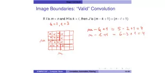
Image Convolution Image Boundaries: “Valid” Convolution If I is m × n and H is k × ℓ , then J is ( m − k + 1 ) × ( n − ℓ + 1 ) COMPSCI 527 — Computer Vision Correlation, Convolution, Filtering 14 / 26

Image Convolution Image Boundaries: “Full” Convolution If I is m × n and H is k × ℓ , then J is ( m + k − 1 ) × ( n + ℓ − 1 ) [Pad with either zeros or copies of boundary pixels] COMPSCI 527 — Computer Vision Correlation, Convolution, Filtering 15 / 26

Image Convolution Image Boundaries: “Same” Convolution If I is m × n and H is k × ℓ , then J is m × n COMPSCI 527 — Computer Vision Correlation, Convolution, Filtering 16 / 26

Filters Filters • What is convolution for? • Smoothing for noise reduction • Image differentiation • Convolutional Neural Networks (CNNs) • . . . • We’ll see the first two next, CNNs later • Smoothing and differentiation are examples of filtering : Local, linear image → image transformations COMPSCI 527 — Computer Vision Correlation, Convolution, Filtering 17 / 26

Filters Smoothing for Noise Reduction • Assume: Image varies slowly enough to be locally linear • Assume: Noise is zero-mean and white x x x x x x x x x x x x x x x x x x x x x x x x x 1/5 COMPSCI 527 — Computer Vision Correlation, Convolution, Filtering 18 / 26

Filters 2 Dimensions: The Pillbox Kernel COMPSCI 527 — Computer Vision Correlation, Convolution, Filtering 19 / 26

Filters Issues with the Pillbox COMPSCI 527 — Computer Vision Correlation, Convolution, Filtering 20 / 26

Filters The Gaussian Kernel COMPSCI 527 — Computer Vision Correlation, Convolution, Filtering 21 / 26

Filters Gaussian versus Pillbox COMPSCI 527 — Computer Vision Correlation, Convolution, Filtering 22 / 26

Filters Truncation u 2 + v 2 G ( u , v ) = e − 1 σ 2 2 • The larger σ , the more smoothing • u , v integer, and cannot keep them all • Truncate at 3 σ or so COMPSCI 527 — Computer Vision Correlation, Convolution, Filtering 23 / 26

Filters Normalization u 2 + v 2 G ( u , v ) = e − 1 σ 2 2 • We want I ∗ G ≈ I • For I = c (constant), I ∗ G = I • Normalize by computing γ = 1 ∗ G , and then let G ← G /γ COMPSCI 527 — Computer Vision Correlation, Convolution, Filtering 24 / 26

Separable Convolution Separability • A kernel that satisfies H ( u , v ) = h ( u ) ℓ ( v ) is separable • The Gaussian is separable with h = ℓ : u 2 + v 2 2 G ( u , v ) = e − 1 2 ( u σ ) g ( u ) = e − 1 = g ( u ) g ( v ) with σ 2 2 • A separable kernel leads to efficient convolution: h k � � J ( r , c ) = H ( u , v ) I ( r − u , c − v ) u = − h v = − k h k � � = h ( u ) ℓ ( v ) I ( r − u , c − v ) u = − h v = − k h h � � = h ( u ) φ ( r − u , c ) where φ ( r , c ) = ℓ ( v ) I ( r , c − v ) u = − h v = − h COMPSCI 527 — Computer Vision Correlation, Convolution, Filtering 25 / 26

Separable Convolution Computational Complexity General: J ( r , c ) = � h � k v = − k H ( u , v ) I ( r − u , c − v ) u = − h Separable: J ( r , c ) = � h u = − h h ( u ) φ ( r − u , c ) where φ ( r , c ) = � h v = − h ℓ ( v ) I ( r , c − v ) Let m = 2 h + 1 and n = 2 k + 1 General: About 2 mn operations per pixel Separable: About 2 m + 2 n operations per pixel Example: When m = n (square kernel), the gain is 2 m 2 / 4 m = m / 2 With m = 20: About 80 operations per pixel instead of 800 COMPSCI 527 — Computer Vision Correlation, Convolution, Filtering 26 / 26