Lecture 10. Simple linear regression 2020 (1) Using one r.v. to - PowerPoint PPT Presentation
Lecture 10. Simple linear regression 2020 (1) Using one r.v. to predict another X and Y are random variables. What is the best linear predictor b 0 + b 1 X of Y ? Prediction error is e = Y ` b 0 ` b 1 X . For the best predictor, there is
Lecture 10. Simple linear regression 2020
(1) Using one r.v. to predict another X and Y are random variables. What is the best linear predictor b 0 + b 1 X of Y ? Prediction error is e = Y ` b 0 ` b 1 X . For the ’best’ predictor, there is zero covariance between e and X , cov( X; Y ` b 0 ` b 1 X ) = cov( X; Y ) ` b 1 var( X ) = 0, so b 1 = cov( X; Y ) = var( X ).
(2) Using one r.v. to predict another Imposing the condition E ( b 0 + b 1 X ) = E ( Y ) gives b 0 = E ( Y ) ` b 1 E ( X ). The prediction can be written Y = E ( Y ) + b 1 [ X ` E ( X )] b We can express the relationship between X and Y as Y = b 0 + b 1 X + e , where b 0 is the predicted value of Y when X = 0.
(3) Prediction error variance Because there is zero covariance between e and X , var( Y ) = var( b 0 + b 1 X ) + var( e ) First term on the right is b 2 1 var( X ) = cov( X; Y ) 2 = var( X ). The prediction error variance is therefore var( e ) = var( Y ) ` cov( X; Y ) 2 var( X ) An alternative expression is (1 ` 2 ) var( Y ), where is the correlation between X and Y .
(4) Regression regress v.i. to go back: to recede: to return to a former place or state: to revert. Tall fathers tend to have tall sons, but average height of sons of tall fathers is less than average height of the fathers. The heights ’regress’ towards the population mean. The prediction equation Y = b 0 + b 1 X is usually called the regression equation, and b 1 the regression coe‹cient.
(5) Parent-o¸spring regression Trait is measured on o¸spring ( Y ) and parents. Mid-parent value ( X ) is the average of the two parental values. According to genetic theory, cov( X; Y ) = 1 var( X ) = 1 2 V A ; 2( V A + V E ) Regression coe‹cient (o¸spring on mid-parent) is b 1 = cov( X; Y ) = var( X ) = V A = ( V A + V E ) ; the heritability of the trait.
75 height of child 70 65 60 64 66 68 70 72 74 height of mid−parent (inches)
(7) Sampling Usually (co)variances are estimated from a sample ( X 1 ; Y 1 ) ; ( X 2 ; Y 2 ) ; : : : ; ( X n ; Y n ) from a bivariate distn. Notation: S xx is the corrected sum of squares for X 1 : : : X n . S yy is the same, for Y 1 : : : Y n . S xy is the corrected sum of products P ( X i ` — X )( Y i ` — Y ) Sample variance S xx = ( n ` 1) and sample covariance S xy = ( n ` 1) provide unbiased estimates of var( X ) and cov( X; Y ). Regression coe‹cient is estimated by ^ b 1 = S xy =S xx .
(8) Simple example Blood pressure was measured on a sample of women of di¸erent ages. Ages were grouped into 10-year classes, and mean b.p. calculated for each age class. Age class (yrs) 35 45 55 65 75 b.p. (mm) 114 124 143 158 166 Model for the dependence of Y (b.p.) on X (age): Y i = b 0 + b 1 X i + e i ; i = 1 : : : n Errors (residuals) e 1 : : : e n are independently distd with zero mean and constant variance ff 2 . Residuals e i are prediction errors, and ff 2 is the prediction error variance (residual variance).
(9) Blood pressure data 170 160 150 140 130 120 110 35 45 55 65 75
(9) Blood pressure data 170 160 150 140 130 120 110 35 45 55 65 75
(10) Calculating slope X = 55, — — Y = 141. Deviations from mean: X : ` 20 ` 10 0 10 20 Y : ` 27 ` 17 2 17 25 S xx = 1000, S yy = 1936, and S xy = 1380. Estimated regression coe‹cient (slope): ^ b 1 = 1380 = 1000 = 1 : 38 (mm/year)
(11) The intercept estimate Equation of the regression line is Y ` 141 = 1 : 38 ( X ` 55) ; or Y = 65 : 1 + 1 : 38 X Slope of the regression line is ^ b 1 = 1 : 38 mm/year, or an average increase of 13.8 mm per decade. The intercept (^ b 0 = 65 : 1) is the predicted value of Y when X = 0. (In this case, an extrapolation far outside the range of the data). To plot the line (manually): Calculate predicted values at two convenient values of X and draw the line joining these two points, e.g. ( X = 35, ^ Y = 113 : 4) and ( X = 75, ^ Y = 168 : 6).
END OF LECTURE
Lecture 11. Residuals and ˛tted values 2020
(12) Fitted values and residuals 170 160 150 140 130 120 110 35 45 55 65 75
(13) Residuals, ˛tted values Values of Y predicted by the regression equation at the data values X 1 : : : X n are called ˛tted values (^ Y ). Di¸erences between observed and ˛tted values ( Y ` ^ Y ) are called residuals. X Y Fitted Residual 35 114 113.4 +0.6 45 124 127.2 ` 3.2 55 143 141.0 +2.0 65 158 154.8 +3.2 75 166 168.6 ` 2.6
(14) Analysis of variance Deviation from the mean can be split into two components: Y i ` — Y = (^ Y i ` — Y ) + ( Y i ` ^ Y i ) Total sum of squares also splits into two components: P ( Y i ` — P (^ P ( Y i ` ^ Y ) 2 Y i ` — Y ) 2 Y i ) 2 = + Total = Regression + Residual Regression SSQ is the corrected sum of squares of the ˛tted values. It simpli˛es to S 2 xy =S xx . Residual SSQ is the sum of squared residuals.
(15) ANOVA calculation Total sum of squares: S yy . Regression sum of squares: S 2 xy =S xx . Residual sum of squares is obtained by subtraction. S 2 ( S yy ` S 2 S yy = xy =S xx + xy =S xx ) Total = Regression + Residual
(16) ANOVA calculation For the blood pressure data, S xx = 1000, S xy = 1380, S yy = 1936. Regression SSQ = 1380 2 = 1000 = 1904 : 4. Residual SSQ = 1936 ` 1904 : 4 = 31 : 6. These calculations are usually set out in an analysis of variance (ANOVA) table.
(17) Analysis of variance table Source Df Sum Sq Mean Sq Regression 1 1904.4 1904.40 Residual 3 31.6 10.53 Total 4 1936.0 Regression SSQ S 2 xy =S xx has one degree of freedom. With a sample of size n , total SSQ has n ` 1 d.f., residual SSQ has n ` 2 d.f. Residual mean square S 2 = 10 : 53 estimates ff 2
(18) A check on the arithmetic Here are the ˛tted values and residuals calculated earlier: X Y Fitted Residual 35 114 113.4 +0.6 45 124 127.2 ` 3.2 55 143 141.0 +2.0 65 158 154.8 +3.2 75 166 168.6 ` 2.6 Check that the residual SSQ is the sum of squared residuals. Check that the regression SSQ is the corrected SSQ of the ˛tted values (sum of squared deviations about the mean value of 141).
(19) Testing zero slope hypothesis Null hypothesis H 0 : b 1 = 0 (‘no relationship between X and Y ’) Sampling variance of ^ b 1 is ff 2 =S xx . q S 2 =S xx is the estimated s.e. of ^ E = b 1 . Under H 0 , ^ b 1 =E has a t distn with n ` 2 d.f.
(20) Testing zero slope hypothesis For blood pressure data, q E = 10 : 53 = 1000 = 0 : 1026, t = 1 : 38 = 0 : 1026 = 13 : 45 with 3 d.f. Tables of the t distn give P < 0 : 001 (two-sided test). Hypothesis is ˛rmly rejected.
Interval estimate for slope parameter Upper 2.5% point for t with 3 d.f. is k = 3 : 182. 95% interval estimate for b 1 is ^ ˚ ( k ˆ E ) b 1 1.38 3.182 0.1026 (between 1.05 and 1.70). Alternative formula: ( t ˚ k ) E , where t is the calculated t statistic. two-sided test at 5% level signi˛cant m end-points of 95% interval have the same sign
END OF LECTURE
Lecture 12. F test, diagnostics, cause and e¸ect, and the lm function 2020
(22) An additional assumption So far, residuals have been assumed uncorrelated, with zero mean and constant variance ( ff 2 ). The results of slides 19-21 (previous lecture) and slide 24 below require the stronger assumption that the residuals are normally distd. (If the sample is reasonably large, the stronger assumption may not be required. The central limit theorem may come to the rescue.)
(23) The F distribution S 2 1 and S 2 2 are independent estimates of variance ff 2 , with degrees of freedom n 1 and n 2 . Distn of S 2 1 =S 2 2 is called the F distn with n 1 and n 2 degrees of freedom Special case: when n 1 = 1, the distn is that of t 2 , where t has a t distn with n 2 d.f.
(24) F test for zero slope Source Df Sum Sq Mean Sq F ratio Regression 1 1904.4 1904.40 180.8 Residual 3 31.6 10.53 Total 4 1936.0 Anova F statistic is the square of the t statistic. H 0 is rejected for large values of F (one-sided test, equivalent to two-sided t test). For b.p. data, F = 180.8 with 1 and 3 d.f. Tables of F with 1 and 3 d.f. show this to be highly signi˛cant ( P < 0 : 001).
(25) Diagnostics Inspect residuals for evidence that model assumptions do not hold. Plot residual against predictor variable or ˛tted value. Plots may show evidence of systematic discrepancy, due to inadequacies in the model, or an isolated discrepancy, due to an ‘outlier’. An outlier has an ‘unusually’ large residual. If possible, a reason should be found. Outliers may sometimes be rejected, cautiously.
(26) Cause and e¸ect A correlation between X and Y does not necessarily imply that a change in X causes a change in Y . The link may be between X and Z , and between Z and Y , where Z is a third (unobserved) variable. For example, a correlation between birth rate and tractor sales may arise simply because both variables are increasing over time.
(27) Regression in R age <- c(35, 45, 55, 65, 75) bp <- c(114, 124, 143, 158, 166) fit <- lm(bp ˜ age) summary(fit) anova(fit) Interval interval for slope parameter: confint(fit, parm = 2)
(28) Summary output > summary(fit) Residuals: 1 2 3 4 5 0.6 -3.2 2.0 3.2 -2.6 Coefficients: Estimate Std. Error t value (Intercept) 65.10 5.8284 11.17 age 1.38 0.1026 13.45 Multiple R-squared: 0.9837 F-statistic: 180.8 on 1 and 3 DF
Recommend
More recommend
Explore More Topics
Stay informed with curated content and fresh updates.
