LEARNING REGRESSION TREES from Time-Changing Data Streams Bla - PowerPoint PPT Presentation
LEARNING REGRESSION TREES from Time-Changing Data Streams Bla Sovdat August 27, 2014 THE STREAM MODEL Example (adult, female, 3.141, 0.577) Data arrives in the form of examples (tuples) (child, male, 2.1728, 0.1123) (child, female,
LEARNING REGRESSION TREES from Time-Changing Data Streams Bla ž Sovdat August 27, 2014
THE STREAM MODEL Example (adult, female, 3.141, 0.577) Data arrives in the form of examples (tuples) (child, male, 2.1728, 0.1123) (child, female, 2.1728, 1.12) Examples arrive sequentially, one by one (child, male, 149, 1.23) … No control over the speed and order of arrival The underlying “process” that generates stream examples might change ) (non-stationary data) Use a limited amount of memory, independent of the size of the stream (infinite data)
DATA STREAM ENVIRONMENT Requirements of the data stream environment: 1) Process one example at a time, inspect it only once Data stream prediction cycle 2) Use a limited amount of memory 3) Work in a limited amount of time 4) Be ready to predict at any time Typical use of data stream learner: a) The learner receives a new example from the stream (1) b) The learner processes the example (2, 3) c) The learner is ready for the next example (4) Different evaluation techniques Alfred Bifet and Richard Kirkby. Data Stream Mining: A Practical Approach. 2009.
INTERMEZZO: DECISION TREES Regression tree represents a mapping from attribute space to real numbers Examples are tuples of attribute values Example: ((male,first,adult),no) Each attribute 𝐵 has a range of possible values: 1) Discrete (also “categorial”) attribute: sex with range {male, female} 2) Numeric attribute: temperature with range R (reals) The target attribute is a real number Example Concrete example: Tom Mitchell. Machine Learning. McGraw Hill. 1997.
INTERMEZZO: CART Famous batch learner for regression trees Start with a set of examples 𝑇 = ( 𝒚 𝟐 , 𝑧 1 , 𝒚 𝟑 , 𝑧 2 , … , ( 𝒚 𝒐 , 𝑧 𝑜 )} , i.e., the training set Each example is of the form ( 𝐲 , 𝑧 ) , where 𝒚 = ( 𝑤 1 , 𝑤 2 , … , 𝑤 𝑏 ) Pick the attribute 𝐵 that maximizes standard deviation reduction (SDR) Partition the set 𝑇 according to the attribute 𝐵 𝐵 = arg max 𝑡𝑡𝑡 ( 𝐵 ) 𝐵 Recursively apply the procedure on each subset 𝑒 1 𝑡𝑡𝑡 𝐵 = 𝑡𝑡 𝑇 − � | 𝑇 𝑗 | 𝑡𝑡 𝑇 = | 𝑇 | � ( 𝑧 − 𝑧 � ) 2 | 𝑇 | 𝑡𝑡 ( 𝑇 𝑗 ) 𝒚 , 𝑧 ∊𝑇 𝑗=1 � = 1 𝑇 𝑗 = ( 𝒚 , 𝑧 ) ∈ 𝑇 𝐵 𝒚 = 𝑏 𝑗 } 𝑧 | 𝑇 | � 𝑧 ( 𝒚 , 𝑧 ) ∊𝑇 L. Breiman, J. Friedman, C.J. Slone, R.A. Olshen. Classification and Regression Trees. CRC Press. 1984.
A PROBLEM Let’s modify CART to a streaming setting Data is not available in advance, and we only see a (small) sample of the stream When and on what attribute to split? What attribute is “the best” relative to the whole stream? Idea: Apply Hoeffding bound to confidently decide when to split
SIMPLIFIED HOEFFDING BOUND Well-known result from probability, also known as additive Chernoff bound, proved by Wassily Hoeffding Many applications in theoretical computer science (randomized algorithms, etc.) and machine learning (PAC bounds , Hoeffding trees, etc.) Theorem (Hoeffding, 1963) . Let 𝑌 = 𝑌 1 + 𝑌 2 + ⋯ + 𝑌 𝑜 be a sum of independent bounded random variables, with 𝑏 ≤ 𝑌 𝑗 ≤ 𝑐 , and let 𝑆 = 𝑐 − 𝑏 . Then ( − 2𝑜𝜁 2 Pr [ 𝑌 − 𝐹 [ 𝑌 ] ≥ 𝜁𝑜 ] ≤ exp 𝑆 2 ) The result is independent of the distribution Randomized Quicksort does at most 48 𝑜 log 𝑜 comparisons “with high probability” Wassily Hoeffding. Probability Inequalities for Sums of Bounded Random Variables. Journal of the American Statistical Association. 1963. Rajeev Motwani, Prabhakar Raghavan. Randomized Algorithms. Cambridge University Press. 1995.
APPLYING THE HOEFFDING BOUND Let 𝐵 1 and 𝐵 2 be the best and the second-best attributes (i.e. attributes with highest SDRs) Let 𝑇 𝐵𝐵 and 𝑇 𝐵2 be estimated standard deviation reductions, computed from 𝑜 examples, for attributes 𝐵 1 and 𝐵 2 If 𝑇 𝐵2 < 1 − 𝜁 , then 𝑡𝑡𝑡 ( 𝐵 2 )/ 𝑡𝑡𝑡 ( 𝐵 1 ) < 1 with probability at least 1 − 𝜀 , where 𝑇 𝐵1 log 1 𝜀 ε = 2𝑜 To see this, solve exp ( −2𝑜𝜁 2 ) ≤ 𝜀 for 𝜁 Note that 𝑡𝑡𝑡 ( 𝐵 2 )/ 𝑡𝑡𝑡 ( 𝐵 1 ) < 1 means 𝐵 1 is better than 𝐵 2 , i.e., it is obvious that 𝑡𝑡𝑡 ( 𝐵 1 )/ 𝑡𝑡𝑡 ( 𝐵 2 ) < 1 iff 𝑡𝑡𝑡 ( 𝐵 1 ) > 𝑡𝑡𝑡 ( 𝐵 2 ) , assuming SDRs are positive This is all we need to scale up the CART learner: Each leaf accumulates examples until it is confident it found the “truly best” attribute Elena Ikonomovska. Algorithms for Learning Regression Trees and Ensembles on Evolving Data Streams. PhD thesis. 2012.
FAST INCREMENTAL MODEL TREES log 1 𝜀 ε = Learning: 2𝑜 1) Start with an empty leaf (the root node) The big picture 2) Sort a newly arrived example into a leaf Update statistics, compute SDRs, and compute 𝜁 3) Accumulate examples in the leaf until 𝑇 𝐵2 < 1 − 𝜁 4) 𝑇 𝐵1 Split the leaf: create 𝑡 new leaf nodes a) Predicting: 1) Sort example down the tree, into a leaf Predict the average 𝑧 of examples from the leaf 2) Elena Ikonomovska. Algorithms for Learning Regression Trees and Ensembles on Evolving Data Streams. PhD thesis. 2012.
EXTENSIONS OF THE FIMT LEARNER Handling numeric attributes (histogram, BST, etc.) Stopping criteria (tree size, thresholds, etc.) Fitting a linear model in leaves (unthresholded perceptron) Handling concept drift (with Page-Hinkley test)
REGRESSION TREES IN QMINER Syntactically no difference between regression and classification (almost) A variant of the FIMT-DD learner available in QMiner The learner exposed via QMiner Javascript API Pass algorithm parameters and data stream specification in JSON format Several stopping and splitting criteria Change detection mechanism, using Page-Hinkley test Can export the model anytime (XML and DOT formats supported) Usage examples available on GitHub The algorithm expects two (learning) or three (predicting) parameters: 1) vector of discrete attribute values; 2) vector of numeric attribute values; 3) target variable value (not needed for prediction)
REGRESSION TREES IN QMINER // algorithm parameters // describe the data stream var algorithmParams = { var streamConfig = { "gracePeriod" : 300, "dataFormat" : ["A", "B", "Y"], "splitConfidence" : 1e-6, "A" : { "tieBreaking" : 0.005, "type" : "discrete", "driftCheck" : 1000, "values" : ["t", "f"] // process the stream "windowSize" : 100000, }, while (!streamData.eof) { "conceptDriftP" : false , "B" : { /* parse example */ "maxNodes" : 15, "type" : "discrete", ht.process(vec_discrete, vec_numeric, target); "regLeafModel" : "mean" "values" : ["t", "f"] } "sdrThreshold" : 0.1, }, "sdThreshold" : 0.01, "Y" : { // use the model "phAlpha" : 0.005, "type" : "numeric" var val = ht.predict(["t", "f"], []); "phLambda" : 50.0, } "phInit" : 100, }; }; // export the model ht.exportModel({ "file" : "./sandbox/ht/model.gv", "type" : "DOT" }); // create a new learner var ht = analytics.newHoeffdingTree(streamConfig, algorithmParams);
REGRESSION TREES IN QMINER The algorithm is pretty fast: tens of thousands of examples per second Scales poorly with the number of attributes (quadratic in 𝑏 ) When using information gain as attribute selection criterion, needs 𝑃 ( 𝑜𝑏 2 𝑑 ) time Numeric attribute discretization is expensive (both space and time) Would love to get feedback from people From now on: Change the algorithm as needed
THE END Been flirting with NIPS 2013 paper A completely different approach to regression tree learning Essentially boils down to approximate nearest neighbor search Very general setting (metric-measure spaces) Strong theoretical guarantees Samory Kpotufe, Francesco Orabona. Regression-tree Tuning in a Streaming Setting. NIPS 2013.
Recommend
More recommend
Explore More Topics
Stay informed with curated content and fresh updates.
